
for
Cosmic
Fields
 Summary
The presently disparate cosmic fields of
dark energy, dark matter, visible or ordinary matter, quantum electrodynamics, and
gravitation are examined by compressible energy flow theory and verifiable
explanatory compressibility patterns are found.
For example, it is possible to fit thermodynamic equations of state for
each field.
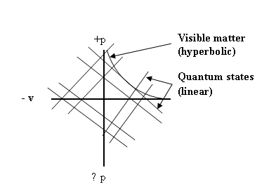
These cosmic equations of state also display
a remarkable symmetry, except for one set of quantum linear states on the pv energy diagram which intersect at the
origin point where there is a curious physical discontinuity.
Shock wave condensations are proposed for
the origin of ordinary matter; the strong shock process for the baryons and
hadrons, and the weak shock option for the leptons and electron. The mass ratios
of the elementary particles of matter are found to fit theoretical compressibility predictions
to within about 1%.
Cosmic state interactions and
transformations are discussed.
Contents
1.0 Introduction
2.0 Outline of Compressible Fluid Flow
3.0 The
3.1 Visible Matter
3.2 Quantum Fields and
Electromagnetism
3.3
Dark Matter
3,4
Dark Energy
3.5
Gravitational Field
4.0 Interactions and Transformations between
States
5.0 The Transformation of
Visible (Baryonic) Matter to Dark
Matter May
Yield an Accelerated Cosmic Expansion
6.0 The Problem of the
Discontinuity at the pv-graphical Point of Origin
7.0 Cosmology, Empirical
Science and an Integrated World View
8.0 Summary
References
Appendix A.
Maxwell’s Electromagnetic Waves and Compressible Flow
Appendix B. Summary of a Universal Physics
1.0 Introduction
At present, the
cosmic fields – dark energy (68.3%), dark matter (26.8%), ordinary baryonic
matter (4.9%), electromagnetic and quantum
fields, and gravitation-- are
partially understood, and they remain
mostly separate theoretically or
conceptually.
We offer an outline of the concept of compressible
fluid flow ( compressible energy flow) as a potential unifying principle for
physical cosmology.
Some previous
work towards this goal [1,2,3] has shown that basic quantum concepts, such
as Planck’s constant, the quantum wave function, the de Broglie wave/particle
equation and so on, can be expressed in
terms of the formalism of compressible fluid flow. In addition, the mass ratios of the
elementary particles of matter can be derived from compressible flow shocks and
their compression ratios – the strong
shock for the hadrons and the weak shock for the leptons.
Here we shall
attempt to incorporate the cosmic fields
into compressible Equations of State. We shall approach this with a brief
review of compressible flow fundamentals with emphasis on examples of how the theory fits various physical fields.
Naturally, such
an attempted overview of intricate and developed fields must be tentative, and
the present approach is offered as such.
2.0 Outline of Compressible Fluid Flow
The following is
a listing of some relevant basic compressible flow principles. For more complete treatment see texts on compressible fluid flow or
gas dynamics.[3, 4,5,6.7.8].
 2.1 Steady State Energy
Equation
2.1 Steady State Energy
Equation
c2 = co2 −
V2/n
(1)
where c is the
local wave speed, co is the static [i.e at V = 0] or maximum wave
speed, V is the relative flow speed, n is the number of ways the energy of the
flow system is divided (i. e. the number
of degrees of freedom) of the system and [
n = 2/(k− 1), where k = cp/cv
is the’ adiabatic constant’ or ratio of specific heats.]
Here, ‘relative’
means referred to any (arbitrarily) chosen physical flow boundary. The equation is for unit mass, that
is, it pertains to ‘specific energy’ flow.
The case where V = c = c* is called the critical state. The ratio (V/c)
is the Mach number M of the flow. The
ratio (V/co) is also a
quantum state variable. The maximum flow velocity Vmax (when c =
0) is the escape speed to a vacuu:
Vmax = √ n co.
2.2 Unsteady State Energy
Equation
c2 = co2
– V2/n – 2/n (dφ/dt)
(2a)
where φ is
a velocity potential, and dφ/dx = u
is a perturbation of the relative
velocity. Therefore, in three
dimensions, substituting V for u, we have dφ/dt = V (dx/dt) = Vc, and
c2 = co2
– V2 /n − 2 (cV)/n
(2b)
(See also sect. 3.2 below for far-reaching implications of the 2cV
interaction energy term in quantum state physics).
2.3 Lagrangian Energy
Function L
L = (Kinetic energy) – (Potential energy)
= ( c2+ V2/n) – co2 , and so, from
(2b)
L = − (2cV)/n
(3)
2.4 Equation of State for
Compressible, Ordinary Matter Systems
The equations of state link the thermodynamic quantities of pressure
p, specific volume ( volume per unit mass v = 1/ρ] and temperature T. The
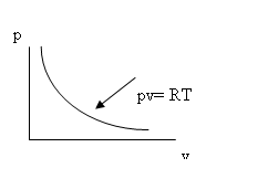
basic equation of state for ordinary
gases is the equilateral hyperbola of the Ideal Gas Law:
pv = RT ; p/ρ = RT = constant
(4)
Equation 4 is
seen to be isothermal (T= constant) .
For adiabatic changes it becomes pvk = constant, where
the adiabatic constant k = cp/cv
is the ratio of the specific heats at constant pressure and at constant volume, respectively.
Here, each point
on the curve presents the values for a particular pressure and volume pair and shows how the two relate to each other
when one or the other is changed. In
this hyperbolic equation, the product of the two -- i.e. the pv- energy -- has a constant value as set out by the
equation of state.
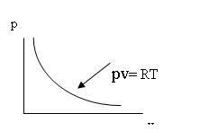
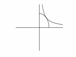
Hyperbolic Equation of State (Ideal Gas Law)
Equations of
State can be formed for gases, liquids
or solids. Here, we shall be concerned mainly with those for the highly
compressible states i.e. for gases.
2.5 Waves and Flow
2.5.1 The
Classical Wave Equation
∆2ψ = 1/c2 [∂2ψ/∂t2] (5)
where ∆2
= ∂2../∂x2 + ∂2.../∂y2
+ ∂2../∂z2;
ψ is the wave amplitude, that is, it is the
amplitude of a thermodynamic state variable such as the pressure p or the
density ρ. The local wave speed is
c.
The general
solution of (5) is
ψ = φ1 (x – ct) + φ2
( x+ ct)
(6)
Equation 6 is a
linear, approximate equation for the case of low-amplitude waves
in which all small terms (squares, products of differentials, etc.) have been
dropped.
The natural
graphical representation of steady state compressible flows and their waves is
on the (x,t), or space-time
diagram.
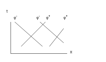
The classical
wave equation corresponds to isentropic conditions. It represents a stable,
low-amplitude wave disturbance, such as an acoustic–type wave.
Unsteady State (
Accelerating) Compressible Flow
In compressible
flow theory, forces, when
present, introduce a curvature of the
characteristic lines for velocity on the space-time or xt-diagram. Space- time
curvature thus indicates velocity acceleration and the presence of force .
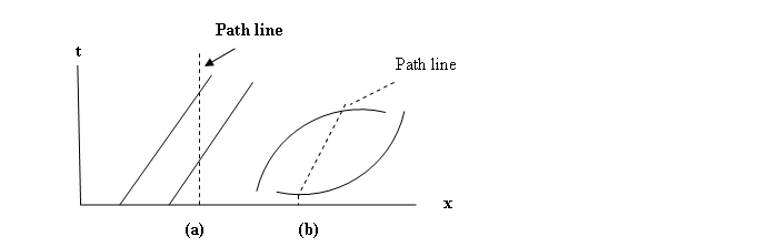
(a) Straight characteristics and path
lines show steady flow and absence of force.
(b) Curved characteristics and path lines show
acceleration and presence of force
In the case of
compressible flow and 3-space (x,y,z) ,
a curved path line dx/dt = v (path) may be ‘transformed away’ to a
straight line Lagrange representation [ dh/dt = 0].
[Note: In General Relativity the analogous
distortion of its 4-space (x,y,z,t) to obtain a force- free representation is a
tensor distortion.
However, it should be noted that
general relativity is a continuous field theory, and, as such, excludes
discontinuities or singularities such as shocks. Therefore, it appears to be
fundamentally incompatible with quantum physics.
On the other hand, compressible
flow as shown below in Section 3.1 on Visible Matter predicts shock
discontinuities as the physical mechanism for the emergence of the elementary
particles of matter by shock compression of an energy flow. Thus, compressible flow is compatible with
quantum theory whereas general relativity is not.]
2.5.2 The Exact Wave
Equation
Ñ2 ψ = 1/c2 ∂2ψ/∂t2
[ 1 + Ñψ ](k + 1) (7)
where k, the
adiabatic exponent, is k = cp/cv = ( n + 2) /n; and ( k +
1 ) = 2( n + 1)/n = 2(co/c*)2. Here, pressure is a function of density
only. This wave is isentropic, non-linear, unstable, and grows to a
non-isentropic discontinuity called a shock wave.
2.5.3
Shock Waves
All finite
amplitude, compressive waves are non-linear and grow in amplitude with time to
form shock waves. These shocks are discontinuities in flow, across which the
flow variables p, ρ, V, T and c change abruptly. (Note p = pressure,
ρ = momentum).
2.5.3.1
Normal Shocks
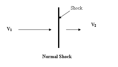
V1 > V2
(8)
p1,
ρ1, T1
< p2, ρ2, T2
(9)
Entropy Change Across Shock:
∆S = S1 – S2 =
− ln(ρ02/ρ01)
(10)
Maximum Condensation Ratio:
ρ1/ρ2
= [n+1]1/2 = Vmax/c*
(11)
2.5.3.2 Oblique Shocks
If the
discontinuity is inclined at angle to the direction of the oncoming or upstream
flow, the shock is called oblique.
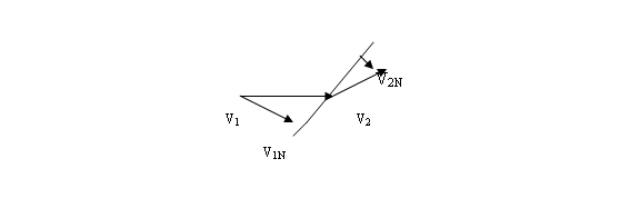
Oblique Shock
V1N > V2N
p1ρ1T1 < p2ρ2
Since the flow V
is purely relative to the oblique shock front, the shock may be transformed to
a normal one by rotation of the coordinates, and the equations for the normal shock
may then be used instead.
2.5.3.3
Strong and Weak Oblique Shock Options: The Shock Polar
For each inlet
Mach number M1 ( = VN1/c), and turning angle of the flow
θ, there are two physical options:
1) the strong shock
( intersection S) with strong compression ratio and large flow velocity reduction (p2 >> p1; V2 << V1, or
2) the weak shock
(intersection W, with small pressure rise and small velocity reduction.
Which of the two
options occurs depends on the boundary conditions: low back i.e. low downstream pressure favours the weak shock
occurrence; high downstream pressure favours the strong shock.
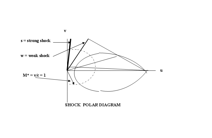
When the turning
angle θ of the oncoming flow is zero, the strong shock becomes the normal
or maximum strong shock, and the weak shock becomes an infinitesimal,
low-amplitude, acoustic wave.
2.6 Types of Compressible
Flow:
a) Steady,
subcritical flow ( e.g. subsonic, V< c), governed by elliptic, non-linear,
partial differential equations.
b) Steady,
supercritical flow ( e.g. supersonic, V1
> c) governed by hyperbolic, nonlinear, partial differential equations.
c) Unsteady
flow (either subcritical or
supercritical). These are wave equations governed by hyperbolic, non-linear,
partial differential equations. They are often simplified to linear approximations,
for example to the classical wave equation (5); if of finite amplitude they
grow to shocks..
The solutions to
the above hyperbolic equations are called characteristic solutions. If linear, they correspond to the
eigenfunctions and eigenvalues of the linear solutions to the various wave
equations of quantum mechanics ( Sect. 3.7), or, equally, to the diagonal
solutions of the matrix equation of Heisenberg’s formulation of quantum
mechanics.
2.7 Wave Speeds
c = [ co2 – V2/n]1/2
(steady flow)
(12)
c = co2 – V2/n
– [(2/n)cV ]1/2 (unsteady
flow)
(13)
c2
= (dp/dρ)s, where s is
an isentropic state.
Since V is
relative, it may be arbitrarily set to zero to give a stationary or “local”
coordinate system moving with the flow; this automatically puts c = co
and transforms the variable wave speed to any other relatively moving coordinate
system.
The shock speed U
is always supercritical (U > c) with respect to the upstream or oncoming
flow V1.
2.8 Wave Speed Ratio c/co and The
Isentropic Thermodynamic Ratios
c/co = [1 -1/n(V/co)2]1/2 = (p/po)1/(n+2) =
(ρ/ρo)1/n = (T/To)1/2 (14)
All the basic thermodynamic parameters of a compressible isentropic flow
are therefore specified by the wave speed ratio c/co. .
2.9 Relativity Effects in
Compressible Flow: In compressible flows all velocities [V or u] are relative only,
and, moreover, the wave speed c is a variable which is dependent on V and n; it decreases for larger
velocities V. and it reaches its maximum
value co at the static state i.e. at
zero flow (V =0).
Interestingly, Equation
(14)
c/co = [1 -1/n(V/co)2]1/2 = (p/po)1/(n+2) =
(ρ/ρo)1/n = (T/To)1/2 (15)
shows that the correction factor for the effect of flow
speed on wave speed c on the right hand side of the equation has the same form as the Lorentz Transformation of special
relativity. If n = 1 the two correction factors become formally
identical.
The differences from
special relativity are that the wave
speed c is now a variable and a
function of the flow velocity V, and that there is the energy partition constant n. Since the wave speeds are low ( c =
334 m/s for air at m.s.l.), the
‘Lorentz’ corrections for physical
compressible systems such as gases are
relatively large. Also, the flow speeds can exceed the wave speed (
supersonic flow), whereas in special relativity theory, the
wave speed c is a constant ( 3 x 10⁸
m/s) which can never be exceeded.
Photon shocks are thus impossible in special relativity, whereas
in compressible flow they furnish a quantum physical theory for the origins of
matter itself via the formation of the
elementary particles of matter at
compression shock discontinuities.
2.10
Wave Stability
Compression waves
are the rule in the baryonic physical world ( i..e. in Quadrant I on the
pressure-volume diagram) where density
waves are always compressive and all
compression waves of finite amplitude grow towards shocks. Here, only acoustic compression waves ( i.e. infinitely low-amplitude
compressions) are stable.
Finite rarefaction
waves and rarefaction shocks are impossible in material gases; only infinitely low-amplitude rarefaction
waves can persist.
We shall see
below that, with elliptical equations of state ( dark matter) and linear
equations of state ( quantum radiation), stable, finite rarefaction waves do
become possible.
2.11
Elliptical Equations of State and Rarefaction Waves
II
![]()
![]()
+p -v
![]()
+v
-p
Elliptical Equation of State favours Rarefaction Waves
and Shocks
The criterion for wave behaviour [4] is the curvature ( dp/dv) of the isentropic equation of state:
1. If d2p/dv2 is > 0 (i.e.
the hyperbolic curve) compression waves form and steepen, while rarefaction waves flatten
and die out. Only compression waves of
infinitely small amplitude (“acoustic” or “sound” waves” ) are stable.
2. If d2p/dv2
is < 0 , ( i.e. the elliptical
curve) rarefaction waves form and
steepen, while compression waves flatten
and die out.
.
We therefore see that ordinary gases are hyperbolic and favour
compression waves and compression shocks. No real gas is known whose equation of state is elliptical and favours
rarefaction waves; but we are now proposing that it is this elliptical relationship
which furnishes the Equation of State
for the Dark Matter of the
universe. ( Section 3.3 below).
We are also proposing that the third option , namely
the linear equation of state, fits
the Quantum state and the
Electromagnetic field. ( Section 3.2 below).
3.0 The Cosmic Fields and Proposed Compressible Equations of State
The main cosmic
fields known to physical cosmology are:
3.1 Ordinary, Visible Matter (4.9% of the cosmos)
3.2
Quantum Fields of the elementary particles of matter, and the electromagnetic field
3.3
Dark Matter (26.8%) of the cosmos)
3.4
Dark Energy ( 68.3 % of the cosmos)
3.5
Gravitation
Of these, the
theory of the quantum
field (including E/M) and the hyperbolic field of ordinary matter are
the most fully developed. In fact, of course, it is from ordinary fluid matter
( liquids and gases) that the concepts of compressible flow have been
developed.
Here, we shall
briefly look at each field in turn from the viewpoint of compressible flow
features and put forward equations of state.
3.1
Ordinary Visible Matter
Ordinary matter consists
of elementary particles held together as atoms and molecules by electromagnetic
forces. Atomic and molecular matter can
exist in three states as gas, liquid and solid. Gases are highly compressible
and all the laws of compressible flow apply to them. Liquids and solids range
from slightly compressible and
distortional to completely incompressible. All three physical states can support waves.
.
First, we examine
the question of What is Matter? Here we shall show that compressible flow
theory gives a direct answer to this crucial question. Clearly, matter is
formed from elementary particles. But a
deeper or more ultimate question is: How
do the elementary particles themselves arise? Here we shall show that, if we start with
energy as a compressible entity, then
the elementary particles can arise naturally from compressible theory as energy
shock wave condensations in a
compressible energy flow.
A Theory of the Origin of
Baryonic Matter: Energy Compressibility in Shock Wave Condensations
We propose
that : All elementary particles of
matter (with the possible exception of the neutrino) are condensed energy forms
produced from hyperbolic equations of state by compression shocks. .
The forms are given
in terms of a simple, integral number n ( n = degrees of freedom of the compressible
energy flow, which is roughly the number
of ways the energy of the system is divided)..
The experimental values of the ratio of the masses to one another are
then related to the maximum theoretical
compression ratio for each compression shock. ( Eq. 16 below). The observed fit is to within 1%.
A. Origin of Hadrons (Baryons and Heavy
Mesons)
Maximum Compression Ratio
mb/mq
= Vmax/c* = [n+1]1/2 (16)
mb is
the mass of any hadron particle, mq
is a quark mass, Vmax = co n1/2 is the escape
speed to a vacuum; that is, it is the maximum possible relative flow velocity
in an energy flow for a given value of n, the number of degrees of freedom of
the energy form, This is a
non-isentropic relationship which corresponds physically to the maximum possible
strong shock. .
Experimental
verification values this hadron mass-
ratio formula is given in Table A below.
Table A) Hadrons (Baryons and
Heavy Mesons)
--------------------------------------------------------------------------------------------
n
n +1 [n+1]1/2 Particle Mass (mb) Ratio to
( MeV) quark mass
_____________________________________________
0 1 1 quark (ud) 310 MeV 1
quark
(s) 505
1
2 3 1.73 eta
(η) 548.8 1.73
3
4
5 6 2.45 rho
(ρ) 776 2.45
6
7
8 9 3 proton
(p) 938.28 3.03 (1)
neutron
(n) 939.57 3.03
Λ (uds) 1115.6 2.97 (2)
Ξo
(uss) 1314.19 2.99 (3)
9 10
3.16 Σ+ (uus) 1189.36 3.17 (2)
10 11
3.32 Ω- (sss) 1672.2 3.31 (4)
Note: Average
quark mass is 310 MeV; (2) Average quark
mass is (u + d+ s)/3 = 375 MeV (3)
Average quark mass is (u+s+s)/3 = 440 MeV;
(4) Average quark mass is 505 Mev.
Comparing column three, the maximum shock compression [n+1]1/2 ],
to the final column “Ratio to quark
mass” we see that they closely agree, so
that the proposed origin of hadrons by strong shock compression theory
expressed in Equation 16 is verified.
B. Origin of
Leptons, Pion and Kaon
mL/me-
=
k/α2 = [(n+2)/n]/α2 = {(n+2)/n] x 137
(17)
where α =
1/11.703 = [1/137]1/2 is the
fine structure constant of the atom , and k is the adiabatic exponent or ratio of
specific heats, k = cp/cv = [(n+2)/n].
Because of the presence of k, this equation
for the mass of the leptons is
thermodynamic and quasi-isentropic.
We propose that the leptons are formed via
the weak shock option( i.e. they involve the reduction in strength of the fine
structure constant [1/137]1/2
The experimental
verification for the lepton mass ratio formula of Eqn. 17 is given in Table B
below.
Table B) Leptons, Pion and Kaon
a
N k = (n+2)/n Particle Mass Ratio Ratio
(MeV) to x 1/137
Electron
__________________________________________________________
1/3 7 Kaon K± 493.67 966.32 7.05
2 2 Pion
π±
139.57 273.15 1.99
4 1.5 Muon μ 105.66 206.77 1.51
- - Electron 0.511 1
Clearly, column 2 values for k ≈ ml/me
(1/137) closely match column 6 for the
mass ratio reduced by 1/137, thus verifying
Equation 17 and the theory that the leptons are formed by weak shock
condensation. .
Summary
The problem of
the origin of the observed mass-ratios of the elementary particles of matter to
one another has here been explained by
the compressible flow expressions to within about 1% of the experimentally
observed values. This grounds the creation of matter in either the strong
compressible shock for the baryons, or in the weak shock option for the
electron and leptons.
. The principle
of the compressibility of energy flow, therefore, would seem to underlie all
material particles and the whole material universe.
Equation of State of Ordinary Liquids and
Gases
The Equation of
State of ordinary compressible cosmic matter ( gas and some liquids) is some
form of the ideal Gas Law, which
a hyperbolic curve on
the pressure volume diagram:
pv
= constant = RT
(a) For isothermal
motions (T = constant) in a real
gas, the equation of state therefore nis just the ideal gas law.
pv = RT or p/ρ = RT
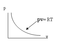
Ideal Gas Law: A hyperbolic equation
of state for Visible matter
(b) For real physical gases
undergoing adiabatic
motions ( i.e.(no heat flow, dQ = 0) the general equation of state is :
pvk = constant
(20)
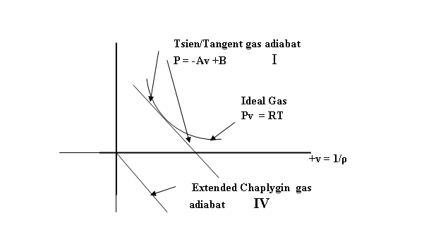
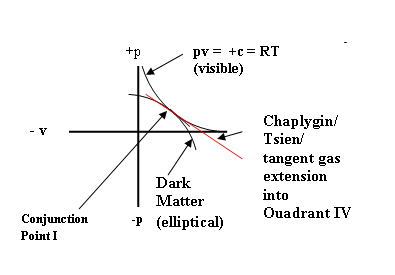
These equations of state
all lie in Quadrant I of the pressure –volume field of Figure 1.
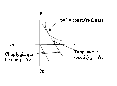
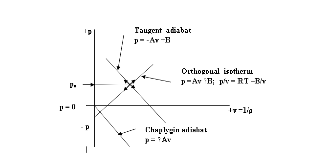
Figure 1.
Pressure-volume in Compressible
Fluids
Quadrant 1:
Real gases and Tsien/Tangent gas (exotic)
Quadrant
IV. :Chaplygin gas and Tsien/Tangent gas (exotic gases)
Equation of State of the Visible Cosmos:
The Hyperbolic Ideal Gas Law
pv = const. = RT
The Hyperbolic Cosmic
Equation of State of Visible Matter
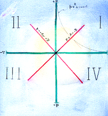
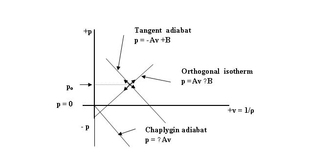
Linear Exotic States: The Tsien/ Tangent Gas and the Chaplygin Gas
These linear
gases were first proposed by Chaplygin [8] and then the tangent gas by Tsien
[7]. In this report we apply them in a much broader sense to
define the linear quantum waves. [ Then,
in conjunction with their orthogonal counterpart, they form a
set of transverse
waves having the form of Maxwell’s electromagnetic wave equations, as
we shall see below in Section 3.2.]
![]()
![]()
![]()
Linear
Chaplygin gas and Linear Tsien/
tangent gas
3.2 Quantum Fields (
principally the Electromagnetic Field or the Field of Quantum Electrodynamics)
These fields describe
the sub-atomic world that produces the elementary particles of matter, the
hadrons and leptons whose assemblages form the
atoms described by the Schrödinger equation. These matters are described by quantum theory which is
highly successful, highly developed, and
highly verified.
We shall not
attempt any comprehensive application of the concept of compressibility of
energy to all the various highly
developed fields of quantum physics. We shall attempt only to show that, in
select examples, compressible wave theory can successfully formulate some
important aspects of quantum theory, implying that compressible action is
physically involved in some cases and at some level. On this basis, for
example, we can see the linear wave equation as a basic descriptor of quantum
electrodynamic phenomena . First the select examples:
The basic quantum
wave function Ψ Is the wave
amplitude. Then, , if the basic quantum
wave function Ψ is defined in a wave se as Ψ = c + v , then the interaction energy term 2cv
from [c + v]2 = c2 + 2cv + v2
appears in most of the
fundamental quantum relationships:
A. The above ‘Extra Energy’or ‘Interaction energy’ term 2cv then yields the following
fundamental quantum relationships:
A) Planck’s Constant, h
For n = 1, if cV = constant energy for each set of
waves, then cV/υ = constant energy per cycle or pulse:
cV/υ = h
cV = hυ = hω/2π = ħω
= ευ
And, for the
complex case:
cV/υ = ħ/i = −iħ
B) De
Broglie Wave/Particle Equation
cV/υ = h
But c/υ
= λ; V(m) = p (momentum), so λp = h, or
p = h/λ
C ) Lagrangian Function, L
L = 2cV
D) Quantum Wave Function
Operators
a) Hamiltonian Energy Operator
cV=
− hυ = −ħω = ε
icV = − ∂../∂t, and so
cV = ħ/i ( ∂../∂t) = +iħ∂../∂t
= Hop
which is the
Hamiltonian energy operator. ( To ensure correct dimensions, it must be applied
to the normalized quantum function ψN).
b) Momentum Operator
cv = hυ = +ħω
= ε
v = (1/c))ħω,
or (m)V = p = (m)(1/c)ħω
Multiplying by i,
we have:
(m)iV = (m)(1/c)
iħω= (m)(1/c) ħ ∂../∂t
So, we have
(m) V = p = -(m)(1/c) iħ ∂../∂t
But,
(1/c) ∂../∂t
= ∂../∂x, and so
(m)V = p = -iħ∂../∂x = pop
which is the
quantum wave operator, ( to ensure correct dimensions, it must be applied to
the normalized quantum function ψN).
E)
Heisenberg Uncertainty Principle
cV = hυ; cV/υ = h
λV = h
But λ =
Δx and V(m) = Δp, so
Δx . Δp ≥ (m) h
which is the
Heisenberg uncertainty principle.
E)
Origin of Elementary Particles of Matter as Shock Condensations in a Quantum
Compressible Flow
This has been dealt with above in Section 2 on the origin of baryonic
material particles and leptons to form
Visible Matter and is repeated here for convenience:
We propose that : All elementary particles of matter (with
the possible exception of the neutrino) are condensed energy forms produced from hyperbolic equations of state by
compression shocks. .
The forms are given in terms of a
simple, integral number n ( n = degrees of freedom of the compressible
energy flow, which is roughly the number
of ways the energy of the system is divided)..
The experimental values of the ratio of the masses to one another are
then related to the maximum theoretical
compression ratio for each compression shock. The observed fit is to within 1%.
A. Origin of Hadrons (Baryons and Heavy Mesons)
Maximum Compression Ratio
mb/mq = Vmax/c*
= [n+1]1/2 (16)
mb is the mass of any
hadron particle, mq is a
quark mass, Vmax = co n1/2 is the escape speed
to a vacuum; that is, it is the maximum possible relative flow velocity in an
energy flow for a given value of n, the number of degrees of freedom of the
energy form, This compression ratio is a
non-isentropic relationship which corresponds physically to the maximum possible
strong shock. .
Experimental verification for this
hadron mass ratio formula is given in Table
A Section 2. above.
B. Origin of
Leptons, Pion and Kaon
mL/me- =
k/α2 = [(n+2)/n]/α2 = {(n+2)/n] x 137
(17)
where α = 1/11.703 is the
fine structure constant, and k is the adiabatic exponent or ratio of specific
heats, k = cp/cv = [(n+2)/n].
Because of the presence of k, this equation
for the mass of the leptons is
thermodynamic and quasi-isentropic.
The leptons are formed via the weak shock option
The experimental verification for
the lepton mass ratio formula is given in Table B Section 2 above.
Summary
Equations 16 and 17 give, uniquely
, an experimentally verified explanation
for the origin of matter as being a
shock condensation from a compressible energetic field., and for the
observed ratios for the masses of the elementary particles of matter. The
principle of the compressibility of energy flow, therefore, appear to underlie
all material particles and the whole material universe.
.
Summary of Compressible Flow and Quantum State Effects: We have been able to
formally relate fundamental
quantum relationships to a single compressible energy pulse term, 2cV.
We have, in
effect, quantized the various energy ‘fields’ represented by 2cV/n for various
values of n, by equating them to the ‘time-like’ condition set by the frequency
υ in the quantum equation hυ = 2cV/n.
(Note that these
equations, as is usual in compressible flow theory, are for ‘specific’ energy,
that is, for unit mass flow. For a
definite particle, the numerical value of the mass is to be inserted; the
dimensions of the equations being not
thereby changed, since in our system, mass (m) is a dimensionless ratio. Thus
for the photon, we have hυ = mγ
cV, where mγ is the relativistic mass of the photon. In
terms of the momentum, p we have
hυ = cp,
which is the de
Broglie equation].
Considering the above relationships, it
seems reasonable to conclude that there
is something fluidic and compressible involved in quantum physics. We suggest that it is the compressible flow
of wave energy (c +V)2 which
underlies this apparent unification of the various quantum relationships listed
above.
Quantum Equation of State : The
Equation of State concept has not at present been applied to all types of quantum fields.
The quantum
reactions produce baryonic matter
composed of elementary particles organized into atoms and molecules. We have
shown above that these elementary particles are associated with compressible
flow shock condensations. The appropriate equations of state for these
particles would seen to be the quantum
wave-particle equations such as the
Schrödinger Equation, the Dirac Equation, the Klein-Gordon wave
equation, the Weyl Equation , the de Broglie wave particle equation.
However, for the
cosmic quantum electrodynamic field
i.e. for electromagnetic radiation, we can propose as
its Quantum Equation of State
the following linear wave equation corresponding to the Tsien/ tangent gas
equation of state and the Chaplygin gas,
but now extended from Quadrant I
into all four Quadrants:
p = ± Av ±B
which, for intercept values A = 1 and B = 0, becomes just
p = ± v
 .
.
− v
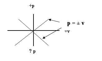
Linear Equation of State p = ±Av ±B
Linear Quantum Fields Equation of State
p = ± v
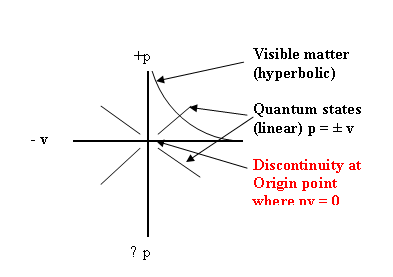
Note
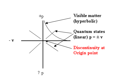
The linear radiation cosmic
state equations p = ± v ,which
pass through the pv-diagram’s Origin Point,
raise a problem of thermodynamic continuity at the point where the wave or flow is postulated to move from
one Quadrant to another. A barrier arises at this origin point where the
specific volume v values and pressure p
must go to zero. Thus, the thermodynamic energy pv equals zero and the thermodynamic temperature
goes to absolute zero.

We must now ask How can
a physical wave of either
rarefaction or compression pass such a
physically discontinuous zero energy state/. Physical i.e. thermodynamic
existence seems impossible in this case.
 These and other questions are troubling
because the linear wave equation of the quantum state is the dynamic link with
the other four cosmic states. In some cases it is the only communication within
and between those states, for example, of
the hyperbolic state with its isolated versions in all four quadrants.
The cosmic symmetry which would unify the various cosmic states via linear
radiation state interaction is broken.
These and other questions are troubling
because the linear wave equation of the quantum state is the dynamic link with
the other four cosmic states. In some cases it is the only communication within
and between those states, for example, of
the hyperbolic state with its isolated versions in all four quadrants.
The cosmic symmetry which would unify the various cosmic states via linear
radiation state interaction is broken.
To repeat,  this is
clear from the fact that a state of absolute zero tempersture is required at
the origin point [since from pv = RT = 0]
. This thermodynamic barrier apparently
prevents any passage or transmission
of a wave or signal through the origin from one quadrant to another. The
geometrical or mathematical symmetry remains, but the physical or
thermodynamic symmetry is broken.
this is
clear from the fact that a state of absolute zero tempersture is required at
the origin point [since from pv = RT = 0]
. This thermodynamic barrier apparently
prevents any passage or transmission
of a wave or signal through the origin from one quadrant to another. The
geometrical or mathematical symmetry remains, but the physical or
thermodynamic symmetry is broken.
[We should perhaps note
that the discontinuity at the origin in the case of the p = ± v wave
equation refers only to the physically real equation. In the case of a purely
mathematical or geometrical equation y = ±
x there would be no such
discontinuity problem since zero values
for the variables are permitted and the equations are then properly seen as mathematically continuous through the
origin point.]
Compressibility and Quantum Electromagnetic Waves : Evidence for Transverse Waves in a Tenuous
Fluid
We have
indicated that some quantum waves are linear and are supported by linear
equation of state. Since there are two
such linear states one of which is adiabatic and the other which is orthogonal
to it and is isothermal, we then have the interesting possibility
that this orthogonal set can support transverse waves in form identical
to Maxwells electromagnetic waves.
There
is a detailed discussion of this in: Appendix
A: Maxwell’s Electromagnetic Waves and Compressible Flow
.
3.3 Dark Matter
Some known characteristics of the dark matter are
as follows :
1. It interacts with
ordinary matter very weakly, and apparently only with the weak force. 2. It causes gravitational lensing of
electromagnetic radiation. 3. It clumps
to form denser entities more readily then ordinary matter. 4. It appears to be denser than ordinary
matter. 5. It makes up about 26.8% of
total cosmic substance. There have been no generally accepted equations of
state for dark matter. The reactions with neutrinos are important but not
considered here.
In the case of
ordinary visible matter, we have stated
above that its state as a cosmic expanding fluid is approximately fitted by the
ordinary hyperbolic gas law pv = RT and
that its adiabatic form is pvk = const. where k is the adiabatic
constant.
Proposed Elliptical Equation of State
We propose an
elliptical equation of state for the dark matter as follows :
P2 /b2 - v2/a2 = a2b2=
Visible Matter pv = const. = RT +p
![]()
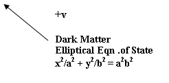
Dark Matter: Elliptical Equation of State
State Properties and Dark Matter Properties: In the elliptical state, rarefaction
waves are demanded and rarefaction shocks are possible. This is seen to
be the opposite or counterpart to
visible matter’s hyperbolic behavior
which requires compression waves and
compression shocks.
Dark matter, if elliptical as theorized, may thus be a ‘form’ of rarefied matter,
interacting with visible matter only via
the weak interaction or possibly by neutrinos.
Its rarefied forms would be the product of rarefied shocks, both the
strong rarefaction shock and weak rarefaction shock, Its stable entities would thus be ‘rarefied forms’, both strong and weak.
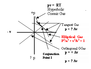
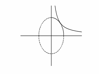
In the graph of the
elliptical equation of state for dark
matter, we have shown the case where dark matter and visible matter contact one
another at a tangent point in
Quadrant This suggests a possible
transformation from one system to another, for example a transformation from visible condensed
matter to invisible rarefied dark matter.
In Sections 4.0 and 5.0 below we
deal with such an interaction in some
detail.
Depiction of the Conjunction of Visible
matter, Dark matter and Linear State matter
3.4 Dark Energy
This form of energy, filling all space, is currently
calculated to constitute about 68.3% of the total observable cosmos..
Because of its property of having negative pressure, it is considered to act to accelerate the expansion of the
cosmos, according to its equation of state:
p/ρ = − 1
How do we depict
this equation of state? First, since the specific density ρ =
1/v, then we have
pv = − 1
While this
negative value for pv energy cannot be depicted in Quadrants I and III, which have pv always
positive, it does fit into Quadrants II and IV as shown.
Negative values for compressible
energy pv = -1 In Quadrants II and
Quadrant IV
The Proposed Dark Energy Equation of State: To derive the corresponding equation of state
of which the −1 value for pv is a point, we note that pv = const is an equilateral
hyperbola. This corresponds to the ideal gas hyperbolic equation of state in Quadrant 1, but now we are in the negative [−pv] Quadrants II and IV,
so that the Equation of State is
(-p)v = const.
It is depicted as
an equilateral hyperbola in Quadrant IV.
Visible matter pv = const. =RT
![]()
.
The dark energy’s
most striking property is its negative pressure, which fills the need
of physical cosmology to explain the observed acceleration in the expansion
rate of the cosmos. The negative
pressure property of Quadrant IV has
already been proposed [9,10,11] via
a linear extension of the
Chaplygin/Tsien/ Tangent Gas from Quadrant I down into Quadrant IV for the
same purpose of explaining the observed
acceleration in the rate of expansion of the cosmos [See also Section 5 below].
[The theoretical possibility of a dark energy
state with negative energy but positive pressure also existing in Quadrant II exists,
but its properties and possibilities for physical
cosmology remain unexplored.]
The dark energy’s
wave forms, being hyperbolic, would be compressive and compression shocks would
be permissible. Low amplitude, acoustic type compression waves of dark energy
would be allowable. Rarefaction waves of
dark energy would be suppressed.
3.5 The Gravitational Field
Characteristics of
Gravitation: The principal characteristics of
gravitational force to be properly
accounted for in a new theory are:
(1) Its universal action on all mass entities, (2) its exclusively attractive nature for
mass, (3 )its weakness relative to the electromagnetic force, and (4) its 1/r2
decline in strength with distance.
The nature of gravitational force:
a) Newtonian and General Relativistic Theories: Newton very successfully
described gravitation as a force acting
on all point masses which fell off in strength as the inverse square of the
distance separating the mass points.
In his General Relativity, Albert Einstein expressed gravitational force as a consequence of motion in a tensorial curved
space time continuum. It was successful
in correctly calculating certain small aberrations from
Newton’s theory, such as the magnitude of the advance in the perihelion of the
planet Mercury. It also correctly describes other astronomical problems so
that General Relativity is the core of the standard theory of physical
cosmology today.
Uniform compressible flow theory and special relativity have some
formal similarities. Both, for example,
yield the Lorentz relationship. [see Sect. 2.10 above ]. General relativity can
be seen as a limiting case of compressible flow when the energy distribution
parameter or degrees of freedom n approaches infinity so that virtual
incompressibility sets in. In this
incompressible limit the field acquires
a tensor character which can be related to non-uniform motion and their
forces.
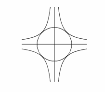
b) Gravity and compressible flow theory:
We propose a circular equation of state for the gravitational
field ( i.e. in all four Quadrants):
Visible matter Hyperbolic Eqn. of State pv = const. = RT = const. = RT +p
P2 + v2 = r2
+v −v
![]()
(1) This equation is
universal with respect to the other fields in that, since it is circular,
it affects all four Quadrants equally,
(2) Because of its negative curvature [ d2p/dv2
= −ve] on the pv diagram, the gravity
waves it carries will be rarefaction
or dilatational ; as such they will exert an attractive force see (Section 2 above, under Wave Stability ) on any baryon mass
object they encounter.
In the above depiction, the radius of the circular
equation of state for gravity has, for
symmetry depiction, arbitrarily been
set at the dimension to give tangency
with the hyperbolic equations of
state for visible matter and dark energy in Quadrants I and IV.
While the simplicity of the circle as an equation of
state for gravity is appealing, still, the conceptual schemes and procedures
for applying it to actual masses and the
other states are still obscure.
Undoubtedly, the concept of ‘centre of mass point’ from Newtonian theory
, i.e. the point at which all the mass of an extended body is concentrated for
calculation of gravitational force, will
be involved. The definition of ‘interaction’ and of an allowable range
of interaction intervals, for example at a tangent point between states as
compared to an intersection point, will need thought.
These and other
implications remain to be explored, and the uncertainty will remain until
observational data are available
to support the proposed circular equation of state.
4.0 Interactions and
Transformations Between Cosmic
States
The possibility would seem
to exist that, at a tangent point or at an intersection, where two states share
identical values of pressure and specific volume, one state may transform into
the other.
Such interaction
concepts should be straightforward for visible matter and quantum fields where
so much work has already been done. Dark
matter and dark energy are more problematical, and gravitation, as has been
pointed out in Section 3.5 above, may be
more difficult still.
Elliptical
(circular) and linear states can (theoretically) exist in all four Quadrants
and assume different or exotic forms as
the numerical values of the state variables change sign. The possibility of
these transformation might be open to
experimental verification on the local scale.
Sharp pressure
fluctuations or pulses would seem necessary for the pv energy point to cross
from one Quadrant to another as, for example , with linear and elliptical or
circular states. In such changes, one
state variable must assume the zero value for the pulse
to cross from one Quadrant to another.
Pressure pulses of large magnitude would probably be of special interest
in triggering state transformation of
this type.
One example of a
cosmic transformation between quadrants would be the proposed Chaplygin gas
transformation from Quadrant 1, with its positive cosmic pressure, to a
Quadrant IV state where the pressure is negative state. This possibility has
been used to explain the observed
acceleration in the rate of expansion of the visible universe [9,10,11].
Hyperbolic states
are confined to one quadrant only. Our
world of baryonic matter can therefore exist in Quadrant I only.
A second class of transformations would be those from one state to
another state within a Quadrant, e.g. from hyperbolic to a tangent or
intersecting linear or elliptical state.
Possibly this transformation type
may be open to experimental verification on the local scale. At tangent points other interactions may
occur. For example, in Quadrant I
quantum state interactions with
baryonic matter interactions must
certainly occur. We explore the
possibility of a
transformation of visible matter
( hyperbolic) into dark matter ( elliptical) in Section 5 below.
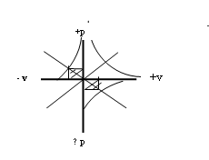
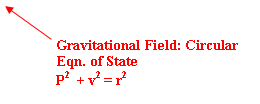
Cosmic Equations of State

![]()
−v
![]()
![]()
Note: In the
above graph, State No.2 – Elliptical
– has been graphed as being circular
simply for reasons of graphical economy, the difference between elliptical and
circular being simply one of a difference in the magnitude of the axial
intercepts a and b for the elliptical
state , and being equal for the case of the
circle.
Interactions: Between gravity (circular)
and all other States.
Between quantum
radiation states ( linear) and all other
States in the same Quadrant
Transformations: From hyperbolic to elliptical in all quadrants, and vice versa
From elliptical in one
quadrant to elliptical in all other quadrants
We see that
hyperbolic forms are fixed to a single
quadrant. This is the case with our world
of visible, baryonic condensed
energy type matter. On the other hand,
rarefied dark matter, if elliptical, as assigned here, might exist in four
Quadrant forms..
5.0 The Transformation of
Visible (Baryonic) Matter to Dark Matter
May Yield an Observed Accelerated Cosmic Expansion
Let us first assume that a
visible to dark matter transformation can occur, and that it yields a change of
state but no change in total rest mass. This leaves us with a need to export any kinetic flow energy in the
transformation system. We can estimate this exportable energy as follows:
K.E.visible = c2
+ V2 +2ncV Assume n = 1
K.E. dark matter = c2
+ V2 + 2ncV Assume
n = − 1, then we have
the numerical difference, or net exportable kinetic flow energy,
in the said transformation:
Δ K.E.transf. = 0 +
0 +4cV= 4cV
Our question now is: Where does the exported energy 4cV go?
 Since the proposed physical change is one
from the compressed energy matter of the visible hyperbolic world to a rarefied
energy of the elliptical dark
matter the physical change must consist of
a pressure drop or rarefaction
pulse. And, reflection will show that,
while such a large pressure drop could take either or both matter states to the
zero pressure line , still their energy
could pass into the negative pressure of
Quadrant IV only for a pulse in which there is no rest mass.
Since the proposed physical change is one
from the compressed energy matter of the visible hyperbolic world to a rarefied
energy of the elliptical dark
matter the physical change must consist of
a pressure drop or rarefaction
pulse. And, reflection will show that,
while such a large pressure drop could take either or both matter states to the
zero pressure line , still their energy
could pass into the negative pressure of
Quadrant IV only for a pulse in which there is no rest mass.
Now, in our equation of state proposed system, the
state with no rest mass is the Linear Wave State, shown in the
Figure as the tangent line from the
interaction
point I running down into Quadrant IV where the 4cV energy is now negative.
This is because p and pv are
negative) in Quadrant IV). This linear wave in Quadrant I is called the the Chaplygin gas or the extended Tsien tangent gas system [7 ,8 ]. In our system it is also the quantum
wave system with equation of state p =
± Av +B].)
Such a transformed flow into negative pressure in Quadrant IV
has already been proposed by a number of researchers [ 9, 10, 11] to explain the observed acceleration in the expansion of the cosmos.
It seems supportive of
our proposed cosmic equations of state and state transformation hypothesis that it should yield a straightforward
physical basis for the negative pressure hypothesis which had little physical basis when it was
first put forward
[9,10,11].
We have thus supplied a physical basis for a possible export of
transformed excess kinetic energy from Quadrant I into Quadrant IV via the linear wave state, where
it supplies negative cosmic pressure and merges with the dark energy pool of
the cosmos.
6.0 The Problem of the Discontinuity at the pv-Graphical Point of
Origin
The simplest
linear cosmic quantum radiation equations of state p = ± v which pass through the pv-diagram’s Origin Point raise a problem of thermodynamic or
physical continuity. A barrier arises at
this origin point where the specific volume v
and pressure p both go to zero.
Thus the thermodynamic energy pv = 0 and the thermodynamic
temperature T = 0. .
We must now ask: Can
a physical wave, of either rarefaction or compression,
pass continuously through such a
physical discontinuous zero energy state? It would seem clear that that they
cannot.
These
questions are troubling because the linear wave equation of the quantum
state is the dynamic link with all the four Quadrants of physical states. . In some
cases this would seem to be the only physical communication within and between
those states, for example, of the
hyperbolic state in Quadrant I with its isolated versions in the other
three. The cosmic symmetry which would unify the various cosmic states via
interaction with linear radiation states
is broken.
To
repeat, zero tempersture is
required at the origin point [since pv =
RT = 0] . This thermodynamic barrier
prevents any passage or transmission of a wave or signal through the origin from
one quadrant to another. The geometrical symmetry is physically and thermodynamically broken.
We should perhaps note here that the discontinuity at the origin
in the case of the p = ± v wave equation refers only to the
physically real equation. In the case of a purely mathematical or geometrical
equation y = ± x there would be no such discontinuity problem since zero values for the variables
are permitted and the equations are then properly seen as mathematically continuous through the
origin point.
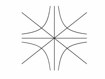
Summary of Cosmic States
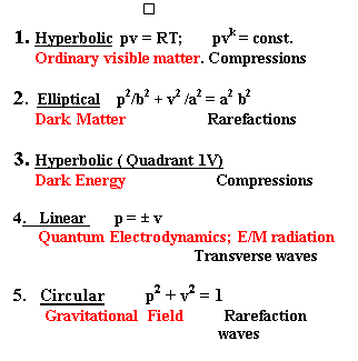
![]()
−v
![]()
Note: In the
above graph, State No.2 –
Elliptical, has been graphed as being circular
simply for reasons of graphical economy, the difference between elliptical and
circular being simply one of a difference in the magnitude of the axial
intercepts a and b for the elliptical
state , and being equal for the case of the
circle.
The understanding
that we have hopefully achieved is that cosmological structures and processes
involve principles of compressible energy flows and their interactions. The
cosmic thermodynamic state equations that we have proposed exhibit a strong
symmetry, especially strong for the linear radiation state which for the case of p = ± v pass symmetrically through the pv-energy
diagram’s origin. And yet, this latter
appealing symmetry is broken by the problem of a continuous wave or radiation
entity being unable to pass through the
thermodynamic barrier of pv = 0 at the origin.
 This raises an unexpected , speculative, but rationally positive possible solution as follows:
1. Cosmic
thermodynamic symmetry is strongly suggested by the compressible equations of state; but this is broken by the discontinuity at
the Origin Point for the case of the linear wave state
p = ± v.
 2. A solution, preserving complete cosmic symmetry, would
require the presence at the Point of Origin of some intrinsically unquantified dynamic entity.
2. A solution, preserving complete cosmic symmetry, would
require the presence at the Point of Origin of some intrinsically unquantified dynamic entity.
3. But, an ‘intrinsically
unquantified dynamic entity’ is, probably what
philosophy would term a
requirement for spirit.
4. Therefore, the
logical argument emerges that “if complete thermodynamic cosmic symmetry
exists, then spirit exists.”
This rather
astonishing but intriguing result is one
for Philosophy and Natural
Theology. It rests logically, of
course, on the appropriateness and
validity of the proposed scheme of cosmic equations of state. This scheme has
been proposed to explain facts of physical cosmology. If the requirement for complete thermodynamic
cosmic symmetry is discarded then the above
theoretical argument is also to be discarded.
The argument, of
course, also cannot be compelling,
since experimental verification is barred, and it is therefore based on postulates and logic, and, any
deletion or defect in these eliminates
the argument. Still, it seems somehow persistent and calling for an answer. The assessment must be
rational with input data from the
three disciplines of science (
cosmology), philosophy and natural theology.
Conclusion
To repeat, if
complete thermodynamic symmetry is desired
for the cosmic equations of state, then the key quantum radiation
equation of state [ p = ±v] lacks continuity at
and across the Origin.
Therefore, if
this thermodynamic cosmic symmetry is
made a requisite, it may require the
introduction, at the origin point discontinuity, of an intrinsically
unquantified dynamism, -which
is philosophically a
spiritual, dynamic entity, -- in order to supply
dynamic continuity through the
origin from one quadrant to another and
so to complete the desired cosmic symmetry.
+p
ХХХ +v -v
A Perfectly Symmetrical
Thermodynamic Cosmos, (Made Possible by
the Presence of ‘Intrinsically
Unquantified Dynamism’ i.e. of Spirit Х ?)
-p
F]’
7.0 Cosmology, Empirical
Science and A More Integrated World View
In the previous Section 6.0
on the physical discontinuity at the
origin, we came to a tentative, very
unusual conclusion which invoked a philosophical
definition. This may reasonably seem unusual in a report on physical cosmology.
Therefore some additional remarks on this point may be in order.
The understanding that we have hopefully achieved is that
cosmological structure, process and cosmic states involve principles of compressible energy
flows and their interactions, and that they therefore show a common structure
and nature. Since compressibility is a
well established field of physical
knowledge, we should thereby have achieved some of the same scientific unification for cosmology. But have we?
For there is an important
difference here. John
Polkinghorne [1below] has pointed out this difference between
cosmology and evolutionary biology from the rest of science. Both of these
scientific fields, he points out, employ all the methods of scientific inquiry except for one,
namely experimental verification, which is denied to them. The cosmos cannot be
experimented on and the evolutionary
past is not experimentally accessible either.
Still, cosmology is a true science and reaches valid insights and
valid and fundamental knowledge. Polkinghorne
also points out that in this respect cosmologists and evolutionary biology methodologically have much in common with philosophy and natural theology, which also reach their understandings [2 below] in the same rational intellectual manner, and yet are likewise denied the satisfaction of
experimental verification.
Thus, in a deep sense, when the results of cosmology are examined
by philosophers and theologians and discussed by them with scientists, all are
then employing the same
intellectual methods and the same tools
of logic and reason and all three stand on the common ground of reason. This necessary communality merits some thought, since in it we may have
the seeds of a wider mutual acceptance and understanding concerning various views of ultimate reality,
It may be useful at this point, then to re-think the situation
from the viewpoint that therein may lie
the beginnings or the elements of
A Re-integrated World View
, one acknowledging the distinctions and the similarities of Science, Philosophy and Natural Theology.
The fields of human
theoretical inquiry
are commonly taken to be Science,
Philosophy, Theology.
1. Science ( excluding Cosmology and Evolutionary Biology) :
Its data and scope concern the
physical world.
Its method is
rational, insightful [2 below],
mathematical and empirical.
Its verification or validation is rational and experimental (empirical).
2. Philosophy: Its data and scope concerns the entire word of
reality i.e .the world of being.
Its method is rational, insightful and logical.
Its verification or
validation is rational, critical and judgmental
3. Natural Theology:
Its data and scope are the data and conclusions from Science and Philosophy
Its method is rational, insightful
and logical i.e. as with philosophy.
Its verification or validation is rational, critical and
judgmental i.e. as with
philosophy.
4.Theology :
See
Lonergan’s “Method in Theology”
[2 below].
5. Cosmology and
Evolutionary Biology
Their data are
observations from the physical world.
Their methods are rational, insightful and mathematical.
Their verification or
validation are those of Philosophy and Natural Theology, namely
rational, critical and judgmental. Scientific
Experimentation is ruled out by their historical
and cosmic nature.
Thus we seem to have the
possibility of a merging of science at its cosmic margins with philosophy and
natural theology, and perhaps therefore the outlines of a Reintegrated World
View. The latter would eventually involve a general understanding and acknowledgement of the separate aims, methods and rational
validation standards for each main field of human intellectual endeavor.
The influence of such a rational and valid Integral World Vew on the multifarious areas of human
civilized activity --artistic, social, economic, governmental
and political--would appear to be undoubtedly beneficial.
Section 7 References:
1. Polkinghorne, John, C., Science
and Creation SPCK, London , 1988
2. Lonergan, S.J., Bernard.
Insight: A Study of Human Understanding.
Philosophical Library Inc., New York, N.Y, 1957. World views surveyed by Lonergan are:
Aristotelian, Galilean, Darwinian, Quantum Indeterminate.
………………, Method in Theology. Herder and Herder, New York, 1972
8.0 Summary
We have shown how a postulated compressible energy field and its flows can fit and unite the main
cosmic fields known to physical
cosmology via symmetrical equations of state. Clearly also, there are many
known facts and aspects not considered here. The proposed equations of state
will have to undergo much critical examination.
In particular, we would emphasize the need for a thorough
thermodynamic analysis for each equation of state and field, and in all
four pv- quadrants in each case. The
entropy behaviour in each instance is also of great interest.
A caveat seems appropriate here. Namely, that the above treatment
using equations of state, although it
touches on exotic and alternative states
and possibilities, is nevertheless
always scientific and physical. These
alternate states in physical cosmology should not be an
invitation to uncritical extrapolation
or imaginative speculation. They do
touch on natural theology and philosophy and such matters have been mentioned in Section 6 above.
[There is one persistent problem that remains. This is the matter
of the broken cosmic symmetry with the simplest linear wave equation of state equations p = ±
v, that is to say with the
set of linear state equations that pass
through the coordinate origin where the pv energy is zero. This problem can raises
extra-scientific questions which are dealt with in Section 6 ].

![]()
−v
![]()
+v −v −p +p +p![]()
![]()

![]()
![]()
1. Power, Bernard A., Unification of
Forces and Particle Production at an Oblique Radiation Shock Front. Contr. Paper N0. 462. American
Association for the Advancement of
Science, Annual Meeting, Washington,
D.C., Jan. 1982.
2. .---------------, Baryon Mass-ratios
and Degrees of Freedom in a Compressible Radiation Flow. Contr.
Paper No. 505. American Association for the Advancement of Science, Annual
Meeting, Detroit, May 1983.
3.
.---------------, Summary of a Universal Physics. Monograph (Private distribution)
pp 92. Tempress, Dorval, Quebec, 1992. (
Appendix B: Summary of a Universal Physics”)
4. .
Shapiro, A. H. The Dynamics and
Thermodynamics of Compressible Fluid Flow. 2 vols. John Wiley and Sons, New York, 1953
5. Courant, R. and Friedrichs, K. O. (1948).
Supersonic Flow and Shock Waves.
Interscience, New York.
6.
Lamb, Horace., Hydrodynamics 6th ed. Dover, New York,
1932.
7.
Chaplygin, S., Sci. Mem. Moscow Univ.
Math. Phys. 21 (1904).
8.
Tsien, H. S. Two-Dimensional Subsonic Flow of
Compressible Fluids, J. Aero. Sci.
Vol. 6, No.10 (Aug., 1939), p.
399.
9.
Bachall, N.A., Ostriker, J.P., Perlmutter, S., and P.J. Steinhardt. The Cosmic
Triangle: Revealing the State of the Universe. Science, 284, 1481 1999.
10.
Kamenshchick, A, Moschella, U., and V. Pasquier. An alternative to
quintessence. Phys. Lett. B 511, 265, 2001.
11.
Bilic, N., Tupper, G.B., and R.D. Violier. Unification of Dark Matter and Dark
Energy: The Inhomogeneous Chaplygin Gas. Astrophysics
, astro- ph/0111325. 2002

![]()
Copyright, Bernard A.
Power, September 2017
Back to Top


Transverse
Waves in a Tenuous Field:
Maxwell’s
Electromagnetic Waves and Compressible Flow
,
Compressibility and Electromagnetic Waves : Evidence for transverse waves in a tenuous
fluid
Here we shall
show that compressible flow theory and the two proposed orthogonal linear equations of state p = ± v can produce transverse waves in a
shear free compressible fluid, so as to fit
with the established transverse nature of electromagnetic waves.
( The
following insert is from UF pages) needs editing to fit in here,,
Material gases, being tenuous fluids, can only support longitudinal waves, that is
to say, waves in which the density variations ±∆ρ are
along the direction of wave propagation. They cannot support transverse waves
in which the density variations would be transverse to the direction of wave
propagation. Its was this inability of a
tenuous medium to transmit the transverse waves of light which led to the
demise of the old luminiferous ether concept.
We now ask: What is the evidence for transverse fluid waves in the Linear Wave
Field with its mutually orthogonal
adiabatics and isotherms?
We consider a
simple pressure pulse ( ±∆p) in the orthogonal wave field:
![]()
A pressure
pulse ( ±∆p) in the Orthogonal Wave Field
The initial or static state
is designated as po. When the pressure pulse ( +∆p) is imposed from outside in some way, the wave
field must respond thermodynamically in two completely orthogonal and
hence two completely isolated ways, namely, by (1) an adiabatic stable
wave along the adiabatic( TG) and (2) by an isothermal stable pulse along the
isotherm (OG).
Spatially, the constant
pressure disturbance ( +∆p) must propagate in the direction of the initial
impulse ,but, since the there are two orthogonal components of the pulse are
the only way for this to take place is
for the two mutually orthogonal components to also be transverse to the direction of propagation of the two
pressure pulses. Vectorially, this
requires an axial wave vector V in the
direction of propagation ( say z) with
the two pulses orthogonally disposed in
the x-y plane. i.e. TG x OG = V which is reminiscent of the Poynting energy
vector S
= E x B in an electromagnetic wave.
E

Electromagnetic Poynting energy /vector
A wave of amplitude ψ traveling in one
direction (say along the axis x) is
represented by the unidirectional wave
equation
dψ/dx = 1/c dψ/dt
Maxwell’s electromagnetic waves
Here, however, in
the case of our adiabatic and isothermal pressure pulses we have two coupled yet isolated
unidirectional waves, and this reminds us of Maxwell’s coupled electromagnetic
waves for E and B, as follows
dEy/dx = (1/c) dB/dt and dBy/dx = (1/c)
dH/dt
where c is the
speed of light, E is the electric intensity and B is the coupled magnetic
intensity.
Maxwell’s E and B vectors are also orthogonal to each
another and transverse to the direction of positive energy propagation.
Therefore, we have formally established in
outline a two component wave system in
theLinear Wave Field with (k = −1) which formally corresponds to the E and B two component orthogonal
system of Maxwell for electromagnetic wave propagation through space in a
continuous medium. His equations for E and B are
Curl E
= ∂Ey/∂x = −(1/c) ∂B/∂t
Curl B = ∂By/∂x = −
(1/c) ∂E/∂t
If we now
designate our Tangent gas as A ( for Adiabatic) and our Orthogonal gas as I (
for Isothermal) then our analogous wave equations would be
Curl A = ∂Ay/∂x = −
(1/c) ∂I/∂t
Curl I = ∂Iy/∂x
= − (1/c) ∂A/∂t
The two systems
are formally identical. Therefore, we propose that the medium in which
Maxwell’s transverse electromagnetic waves travel through space is to be physically identified as a Linear
Wave Field, having the above described thermodynamic
properties for adiabatic and isothermal motions initiated in the wave field and
initiated by pressure pulses ( presumably by accelerated motions of electric
charges.) The compressibility of the wave state now accounts on physical grounds for the finite wave speed ( speed of light), and
in addition wave motions in this
tenuous fluid medium are transverse, as required by the observations..
It is possible to
reduce Maxwell’s two equations UF equations to a symmetrical single wave
equation
∂2E/∂x2 =
(1/c2) ∂2E/∂t2
∂2B/∂x2 =
(1/c2) ∂2B/∂t2
and similarly
with A and I for our Adiabatic/Isothermal
coupled wave in the UF:
∂2A/∂x2 =
(1/c2) ∂2A/∂t2
∂2I/∂x2 =
(1/c2) ∂2I/∂t2
This is not surprising
since the UF with its k = −1 thermodynamic property is the unique compressible fluid which automatically
generates the classical wave equation with its stable, plane waves. The formal
agreement of the UF theory with Maxwell is again striking.
Instead of taking our initial external perturbation as a pressure pulse ( +∆p) we should more realistically, from the physical
standpoint, take it to be a density condensation (s = ( ρ – ρo ) / ρo
= +∆ρ/ ρo).
This will now result in a positive pressure pulse (+∆p) appearing in the adiabatic (TG) phase of the UF but a negative pressure pulse ( −∆p) in the
isothermal or orthogonal perturbation component (OG) . This perturbation is
represented by the two orthogonal sets of arrows on the pv diagram, one
corresponding to +∆p and the other set corresponding to − ∆p.
As the wave progresses the two orthogonal vectors also rotate.
![]()
 S
S
The
physical ambiguity which results from a pressure/density perturbation in the
Orthogonal UF
An oscillating
density perturbation ( ±∆ρ) then results in an axial wave vector
having two mutually orthogonal
components ( adiabatic and isothermal ) in a density perturbation wave. This appears to correspond formally to the
Maxwell electromagnetic wave system with its two mutually orthogonal vectors
for electric field intensity E and
magnetic field intensity B.
We have thus established a case for the
compressible linear wave field being a
cosmic entity which transmits transverse electromagnetic waves through space. A
necessary next step will be to examine the field or state in relation to all the multifarious established facts relating to electromagnetic
radiation.. These must include the nature of electric charge, electrostatic
fields, the compressed fields of moving charges and the resulting magnetic
fields, etc. etc. Preliminary work has indicated that this additional
reconciliation will be successful.
Nite: The appropriate wave
equation for the compressible flow field, from which the quantum shock
compressions that generate the elementary particles of matter are produced,
would seem to be the exact Classical
Wave Equation:
Ñ2 ψ =
1/c2 ∂2ψ/∂t2 [ 1 + Ñψ
](k + 1)
where k, the adiabatic exponent is
cp/cv = ( n + 2) /n; and ( k + 1 ) = 2( n + 1)/n = 2(co/c*)2. Here, pressure is a function of density
only. This wave is isentropic,
non-linear, unstable, and grows to a non-isentropic discontinuity called a
shock wave. It is at these shock
discontinuities that the elementary particles can form – the hadrons at the
strong shock and the leptons at the weak shock option.
In many quantum actions stable waves are involved, such as the electromagnetic waves. For these we propose
the linearised classical wave equation, as follows
∆2ψ = 1/c2 ∂2ψ/∂t2
where ∆2 = ∂../∂x2
+ ∂2../∂y2
+ ∂2../∂z2;
ψ is the wave amplitude, that is, it is the
amplitude of a thermodynamic state variable such as the pressure p or the
density ρ. The local wave speed is
c.
The general solution is
ψ =
φ1x – ct) + φ2( x = ct)
This equation is a linear,
approximate equation for the case of
low-amplitude waves in which all small terms (squares, products of
differentials, etc. have been dropped.
Summary
We have presented examples of a
close conection of compressible flow theory and quantum mechanics fundamental
relationships. We have related the formation of the elementary prticles of
matter to energy condensation occurring in compression shocks in a compressible
flow.
We have
assigned a Linear Equation of State to
the quantum fields of electromagnetic
radiation. This equation has two forms, one being adiabatic and the
other being isothermal. In the case wheer these two ewuations are orthogonal. the
resultant wave would appesr to be
transverse to the direction of motion.. Then, the transverse wave
equations are shown to formally match Maxwell’s electromagnetic equations.
![]()
Copyright, Bernard A.
Power, September 2017
Summary
of a Universal Physics
May 1992
SUMMARY
OF A UNIVERSAL PHYSICS
Bernard
A. Power
Consulting Meteorologist (ret.)
TEMPRESS
©
1992
PREFACE
The central concept of the new unified
theory of physics which is the subject of this book, is that energy flows and
transformations are compressible, and that this single concept makes possible
the unification of the presently separate fields of physics – classical
mechanics, quantum mechanics, nuclear physics, relativity and gravitation.
We may roughly characterize this
compressibility as : (1) the capacity of energy to exist in the form of various
elementary particles having varying concentrations or densities of energy, and
(2) transformations from one particle
form to another take place via energy flows which involve energy compressibility.
The existence of compressibility has very
important physical consequences. For
example, it permits certain supercritical motions to exist which now provide a
long-sought-for physical explanation for the existence of the elementary
particles of matter in their various mass-ratios, for whole ranges of quantum
and nucleqar phenomena, and for their unification with other branches of
physics.
Of course, a new, central scientific
concept, to be valid, must relate in a fundamental way to an enormous range of
scientific topics and experimental data.
The complete exposition of such a new theory in all its details would
obviously be quite impossible to accomplish in a single book, or even in
several; and, given the current high level of development and complexity of
physics, it would not only be far beyond the ability of any one individual, but
would undoubtedly tax the capabilities of a whole team of specialists. Still, any fundamental, new concept must have
a beginning, and beginnings are usually small – hence the present small book
with such an extended scope.
The evidence presented for the general
correctness of the new theory is both
theoretical and experimental.
Theoretically, Section 3 presents a new
physical basis for quantum physics which is compatible with the standard model
in most respects, by making use of the concept of energy waves, and
compressible flows and transformations. The quantum state variables are the
wave speed c and the relative flow velocity V; the normalized quantum wave functions
are c/co and V/co.
The energy of the wave function contains a
new energy term, 2cV, which in turn then grounds all the quantum relationships
on a basis of extreme simplicity – Planck’s constant h, the de Broglie
equation, the Lagrangian function, the quantum operators for momentum and
position, and the Heisenberg uncertainty principle. The entropy is derived from
a basic, compressible energy equation, and this in turn yields the fine
structure constant of the atom α in an extremely simple manner.
Experimentally, the problem of the
mass-ratios of the elementary particles of all matter is explained by the
compressible flow expression [n+1]1/2 to within about 1% of
experimental values. This grounds the creation of matter in either the strong
compressible shock for the baryons, or the weak shock for the electron and the
leptons.
In this book, mass becomes a dimensionless quantity – a measure of the degree of energy
condensation of the various elementary particles of matter.
In section 4, the physical basis for
electric charge is related to compressible vortex motion ; charge is then
related to the entropy and the fine structure constant. The results of the
optical experiments of Michelson and Morley are shown to be consequences of
compressibility. The refractive index in optical media is derived from the
compressibility equation, as well as Fermat’s least-time principle for optical
rays. The experimental discrepancies in
some versions of the Fizeau experiment are explainable as shock phenomena.
In Section 5, the basic relativity
relationships, such as the Fitzgerald contraction factor and the Lorentz
transformations, are shown to be simple consequences of the compressibility
ratios c/co and V/co, which, as mentioned above, are also
the normalized quantum state variables.
In Section 6, the 2cV compressibility
perturbation term is shown to lead to a quantum theory of gravitation; the
nature and physical generation of the quantum of gravity are shown to be
related directly to the generation of the elementary particles of matter by the
strong and weak shock condensations of energy.
Mach’s Principle becomes expressed on the physical basis of
compressibility.
The quantum nature of gravity leads to a
deeply-rooted cosmology in a universe evolving through Unitary → Binary →
Unitary transformations; this process
provides a solution to the current mystery of the so-called ‘missing mass’ or “
dark matter” of the universe.
Experimentally, Section 8 resolves the
conflict over the cosmological constant; that is, it reconciles quantum
predictions of an enormous vacuum energy with the conclusions of astronomy of a
zero energy vacuum and a nearly flat structure for space. The observed early abundance of quasars in
space is explained by the new theory in an experimentally testable
prediction. The A → B transformation of matter yields an
energy-change equation from which the prediction might be tested against energy
requirements for astronomical processes.
Since a new theory cannot be exhaustive,
the present summary aims to present to specialists only a brief overview of
applications and some preliminary results, so as to encourage and assist in a
more detailed examination.
Those already familiar with compressible flow
theory e.g. aerodynamicists, astronomers, meteorologists ( such as the author)
and so on will probably find Section 2 merely a review. Those unfamiliar with
it will hopefully find the Section to be a concise presentation of compressible flow topics which
will provide a key to the application of the new theory to their various
specialties in the later sections.
May 1992
CONTENTS
Section 1 Introduction
Section 2 Compressible Fluid Dynamics
2.1 Steady state energy equation
2.2 Unsteady state energy equation
2.3 Lagrangian energy function L
2.4 Equation of state for compressible
systems
2.5 Waves
2.5.1 Classical wave equation
2.5.2 Exact wave equation
2.5.3 Shock waves
2.5.3.1 Normal shocks
2.5.3.2 Oblique shocks
2.5.3.3 Strong and weak shock options:
The shock polar
2.6 Types of compressible flow
2.7 Compressible flow ratios and parameter k
2.8 Wave speeds
2.9 Wave speed ratios and isentropic ratios
2.10 Graphical depiction of waves and shocks
2.11 Wave stability
Section 3 Quantum Physics
3.0 General
3.1 Compressibility and quantum mechanics
3.2 Basic quantum wave
3.3 Interacting ( non-parallel) quantum waves
3.4 Curved characteristics
3.5 Quantum wave function
3.5.1 Normalized quantum wave function
3.5.2 The specific energy of the wave function
3.5.3 The ‘extra energy’ term 2cV
3.6 The ‘extra energy’ term 2cV yields the
following fundamental quantum
relationships
A) Planck’s constant h
B) de Broglie wave/particle equation
C) Lagrangian function L
D) Quantum wave function operators
E) Heisenberg uncertainty principle
3.7 Quantum wave/particle equations
3.7.1 Schrodinger equation
3.7.2 Dirac equation
3.7.3 Klein-Gordon wave equation
3.7.4 Weyl equation (neutrino)
3.8 Quantum state functions
3.9 Origin of matter and energy
compressibility
A) Baryons
and heavy mesons
B) Leptons,
pion and kaon
3.9.1 Experimental verification of mass-ratio equations
3.9.2 Summary
3.10 Entropy and the mass ratios
3.11 Entropy and the fine structure constant
3.12 Quantum interactions and elementary
particle interactions; Graphical depiction
3.13 Radioactive Decay
3.14 Spin, reflection, particle confinement and
spinors
3.15 Quantum creation and annihilation operators
3.16 The ‘collapse of the wave function’ problem
3.17 Nature of the quantum wave function
3.18 Feynman diagrams and virtual particles
3.19 Dirac delta function
Section 4 Electromagnetism
4.1 The physical basis of electrical charge
4.1.1 Charge as vortex motion
4.1.2 Vorticity at a contact discontinuity
4.1.3 Entropy and electric charge
4.1.4 Entropy and pressure ratio
4.1..5 Compressible potential vortex
4.1.5.1
Compton wave length, λc
4.1.6 Electron vortex pressure
4.1.7 Model of the hydrogen atom:
A)
The rotational vortex
B) Compressible vortex
C) The hydrogen atom: nucleus + electron
4.1.8 de Broglie wavelength. λdeB
4.2 Electrostatic field
4.3 Magnetism: The compressed virtual photon
field of a moving charge
4.4 Electromagnetic radiation
4.5 The photon structure:
4.5.1 Cusp vector field
4.5.2 Photon energy
4.5.3 Photon speed
4.5.4 Relativistic form
4.5.5 Photon spin
4.6 The Michelson-Morley experiment
4.7 Some Optical Effects:
4.7.1 The refractive index N
4.7.2 The Fizeau Effect
4.7.3 Fermat’s Least Time principle for optical rays
4.8 The Sagnac Effect
4.9 The de Broglie equation
4.10 The Periodic Table
Section 5 Relativity: A Compressibility Effect
5.1 Galilean relativity
5.2 Special Relativity:
5.2.1 The Fitzgerald contraction factor
5.2.2 The Lorentz transformations
5.2.3 The relativistic Hamiltonian
5.2.4 The Einstein formulation of special
relativity
5.2.5 Compressibility formulation of special
relativity
5..2.6 Transverse and longitudinal mass
5..3 General relativity
Section 6 Gravitation and Cosmology
6.0 General
6.1 Force in compressibility terms
6.1.1 ‘Longitudinal mass’
6.1.2 Force in pressure gradient terms
6.1.3 Wave speed c
6.2 Derivation and dimensions of the
gravitational constant G
6.2.1 Gravitational wave speed
6.3 The gravitational quantum or gravitino
6.4 Force of gravity in compressibility terms
6.5 Exclusively attractive nature of gravity
6.6 A new force law
6.7 Equivalence of gravitational and inertial
force: Mach’s Principle
6.8 The problem of the cosmological constant
6.9 The ‘flatness’ problem: Ώ equals
unity
6.10 Action-at-a-distance : The experiments of
Aspect et al.
6.11 The hidden mass, or “dark matter”, of the
universe:
6.11.1 The equation of state has two forms
6.11.2 Rarefied or celeston matter
6.11.3 Local pressure lowering in vortices
6.11.4 Quasars in early cosmic times [ p >>p*]
6.11.5 Spiral and elliptical galaxies
6.12 Experimental text of the proposed A →
B transformation: Quasars vs. galaxies
Selected
Bibliography
SUMMARY
OF
A
UNIVERSAL PHYSICS
1.
INTRODUCTION
1.1
The whole of physics –
classical mechanics and thermodynamics, quantum mechanics, electromagnetism,
relativity, gravitation and cosmology – can be unified on the basis of a single,
theoretical principle – the compressibility of energy flows or energy
transformations. This principle thus
introduces a universal physics.
1.2
It is postulated that all
energy transformations and processes involve compressible motions which are governed
by the laws of compressible fluid flow.
1.3 Energy always exists in a definite
physical configuration or ‘form’, such as a massive elementary particle, a wave
pulse, a photon, etc., but never as ‘energy per se’.
1.4
Section 2 is an outline
of some essentials of standard, compressible fluid flow theory. Sections 3 to 6
then apply these to some fundamental topics in quantum physics,
electromagnetism, relativity and cosmology, to show the universality of the new
theory.
2. COMPRESSIBLE FLUID DYNAMICS
2.1 STEADY STATE ENERGY EQUATION
c2 = co2 - V2/n
(1)
where c is the local, compressive wave speed, co
is the static wave speed or maximum wav e speed, V is the relative flow
speed, n is the variety of the energy configuration ( the number of degrees of
freedom) of the system.
Here, ‘relative’ means referred to any (arbitrarily) chosen
physical boundary. The equation is for units mass, that is, it pertains to
specific energy flow.
The case where V = c = c*
is called the critical state. The ratio (V/c) is the Mach number M of
the flow. The ratio (V/co) is
a quantum state variable ( Sects. 2.10b; 3.8). The maximum flow velocity Vmax
(when c = 0) is the escape speed to a vacuum; Vmax = √ n
co.
2.2 UNSTEADY-STATE ENERGY EQUATION
c2 = co2
– V2/n – 2/n dφ/dt
(2)
where φ is a
velocity potential, and dφ/dx = u is the perturbation of
relative velocity. Therefore, in three dimensions, substituting
V for u, we have
dφ/dt = V (dx/dt) = Vc
and
c* = co* - V*/n - 2/n cV
(2b)
(See also sects. 3.6; 6.2; 6.9; and 8.10 for far-reaching
implications of the cV term).
2.3 LAGRANGIAN ENERGY FUNCTION L
L = (Kinetic energy) – (Potential energy)
= ( c2 = V2/n) – co2
, and so, from (2b)
L = - 2cV/n
(3)
2.4 EQUATION OF STATE FOR COMPRESSIBLE SYSTEMS
pv = RT ; p/ρ = RT
(4)
p = pressure, v = volume, 1/v = ρ, the density; R =
gas constant; t = temperature.
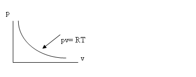
Equation of State
2.5 WAVES
2.5.1 CLASSICAL WAVE EQUATION
∆2ψ = 1/c2 ∂2ψ/∂t2
(5)
∆2 = ∂../∂x2 + ∂2../∂y2 +
∂2../∂z2;
ψ is the wave amplitude,
that is, it is the amplitude of a thermodynamic state variable such as the
pressure p or the density ρ.
The general solution of (5) is
Equation 6 is a linearized, approximate equation for the case of low-amplitude waves in
which all small terms (squares, products of differentials, etc.) have been
dropped. The natural representation
ψ = φ1x – ct) +
φ2( x = ct)
(6)
of compressible flows and their waves is on the (x,t), or
space-time diagram.
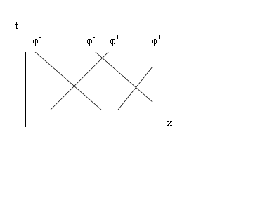
The classical wave equation corresponds to isentropic conditions.
It represents a stable, low-amplitude disturbance, such as an acoustic–type
wave. The exact form follows:
2.5.2 EXACT WAVE EQUATION
Ñ2ψ
= 1/c2 ∂2ψ/∂t2
[ 1 + Ñψ ](k + 1)
(7)
where k, the adiabatic exponent is cp/cv = ( n +
2) /n; and ( k + 1 ) = 2( n + 1)/n = 2(co/c*)2. Here, pressure is a function of density
only. This wave is isentropic,
non-linear, unstable, and grows to a non-isentropic discontinuity called a
shock wave.
2.5.3 SHOCK WAVES
All finite amplitude, compressive waves are non-linear, and steepen
with time to form shock waves. These are
discontinuities in flow, across which the flow variables p, ρ, V, T and c
change abruptly. (Note p = pressure, p
= momentum).
2.5.3.1 NORMAL SHOCKS
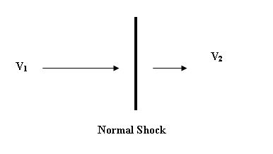
V1 > V2>
P1,
ρ1, T1
< p2, ρ2, T2
ENERGY;
V12/2 + h1 = V22/2 + h2 = ho
(8)
where ho – stagnation enthalpy.
CONTINUITY:
ρ1V1
= ρ2V2
(9)
MOMENTUM:
p1 + ρ1V12 = p2
+ ρ2V22
(10)
EQUATION OF STATE:
h = h(s,p);
S = S(p,ρ)
(11)
PRANDTL’S EQUATION:
V1V2 = c*2
(12)
V1V2 = ρ2/ρ1
(13)
ENTROPY CHANGE ACROSS SHOCK:
∆S = S1 – S2 = -ln(ρ02/ρ01) (14)
MAXIMUM CONDENSATION RATIO:
ρ1/ρ2 = [n+1]1/2
= Vmax/c*
(15)
2.5.3.2 OBLIQUE SHOCKS
If the discontinuity is inclined at angle to the direction of the
oncoming or upstream flow, the shock is called oblique.
Oblique Shock
V1N > V2N
p1ρ1T1 < p2ρ2T2
ENERGY:
[V1N2 – V1N2]
/2 = (n+2)/n [p2/ρ2
– p1/ρ1]
or,
1/2[ V2N2 – V1N2] = cp
[ T1 –T2 ]
(16)
CONTINUITY:
ρ1V1N = ρ2V2N
(
17)
MOMENTUM:
p1 - p2
= ρ2V2N2 – ρ1V1N2
(18)
RANKINE-HUGONIOT EQUATION:
Ρ2/ρ1 = [(n+1)(p2/p1)
+1] / [(n+1) + (p2/p1)]
(19)
PRANDTL EQUATION:
VN1VN2 = c*2 – 1/(n+1) Vmax2
(20a)
V1/c* + c*/V2 = V2/c*
+ c*/V2
(20b)
Since the flow V is purely relative to the oblique shock
front, the shock may be transformed to a normal one by rotation of the coordinates,
and the equations for the normal shock may then be used instead.
2.5.3.3 STRONG AND WEAK OBLIQUE SHOCK OPTIONS: THE
SHOCK POLAR
For each inlet Mach number M1 (
= VN1/c), and turning angle of the flow θ, there are two
physical options:
1) the strong shock ( intersection S) with
strong compression ratio and large flow
velocity reduction (p2 >>
p1; V2 << V1,
or
2) the weak shock (intersection W, with small pressure
rise and small velocity reduction.
Which of the two options occurs depends on the
boundary conditions: low back, or downstream, pressure favours the weak
shock occurrence; high diownsgream pressure favours
the stroing shock.
When the turning angle θ of the oncoming flow is
zero the strong shock becomes the normal or maximum strong shock, and the weak
shock becomes an infinitesimal, low-amplitude, acoustic wave ( described by Eq.
5).
2.6 TYPES OF COMPRESSIBLE FLOW
a) Steady, subcritical ( e.g. subsonic, V< c),
governed by elliptic, non-linear, partial differential equations.
b) Steady, supercritical ( e.g. supersonic, V1 > c) governeddd by
hyperbolic, nonlinear, partial differential equations.
c) Unsteady (either subcritical or supercritical).
These are wave equations governed by hyperbolic, non-linear, partial
differential equations. They are often simplified to linearised approximations,
for example to the classical wave equation (5); if of finite amplitude they
grow to shocks..
The solutions to the above hyperbolic equations are
called characteristic solutions. If
linear, they correspond to the eigenfunctions and eigenvalues of the linear
solutions to the various wave equations of quantum mechanics ( Sect. 3.7), or,
equally, to the diagonalized solutions of the matrix equation of Heisenberg’s
formulation of quantum mechanics.
TWO-DIMENSIONAL,
STEADY, SUBCRITICAL FLOW
(1 – M2)
∂u/∂x + ∂v/∂y =
0
(21)
where M = V/c and c2 = co2
– V2 /n.
Thus equation is elliptical, and reduces by a simple
transformation to the Laplace equation
Ñ2ψ =
0 (22)
TWO-DIMENSIONAL,
STEADY, SUPERCRITICAL FLOW
(M2
– 1) ∂u/∂x - ∂v/∂y = 0
(23)
where M and c are as given in (21).
This equation is hyperbolic and reduces to the
classical wave equation (5) by a simple transformation.
UNSTEADY,
ONE-DIMENSIONAL MOTION
(c2 –
φx2) φxx - 2φxφt
– φtt = 0
(24)
where φ is a velocity potential, i.e. ∂φ/∂x
= u, etc., and c2 = co2 –V2/n –
(2n) dφ/dt.
In linearised form, we have the classical wave
equation in terms of the velocity
potential φ:
Ñ2φ = 1/c2 ∂2φ/∂t2 (25)
2.7 COMPRESIBLE FLOW RATIOS AND PARAMETER K
Vmax/co
= n1/2; Vmax/c* =
(n+1)1/2
(26)
(co/c*)2
= n/(n+1); c/co = [1 –
1/n)(V/co)2
(27)
n =
2/(k-1); k = cp/cv
= (n+2)/n
(28)
2.8 WAVE SPEEDS
c = [ co2
– V2/n]1/2 (steady flow)
(1)
c = [ co2
– V2/n – (2/n)cV ]1/2 (unsteady
flow)
(2)
c2
= kp/ρ = (dp/dρ)s, where s is an isentropic state
(29)
Since V is relative, it may be arbitrarily set to zero
to give a stationary or “local” coordinate system moving with the flow; this
automatically puts c = co and transforms the variable wave speed to
any other relatively moving coordinate system. (See also Sect. 5.2).
The shock speed U is always supercritical (U > c) with
respect to the upstream or oncoming flow V1.
2.9 WAVE SPEED RATIOS AND ISENTROPIC RATIOS
c/co
= [1 -1/n(V/co)2]1/2 = (p/po)1/(n+2) =
(ρ/ρo)1/n = (T/To)1/2 (0)
All the basic physical parameters of a compressible
isentropic flow are therefore specified by the wave speed ratio c/co.
2.10 GRAPHICAL DEPICTION OF WAVES AND SHOCKS
a) Waves, shocks and their various interactions are
depicted in the space-time or x,t-coordinate system, which is also called the
physical plane.
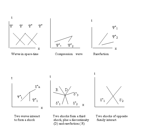
b) State plane representation
On the state (c,V) plane the characteristics Γ±1,2
show as two sets of lines inclined at slopes of +(1/n) and –(1/n). The
normalised state plane has state coordinates (c/o) and (V/co).
It yields all the thermodynamic variables of state from the isentropic ratio
relationships via the wave speed ratio c/co ( Eq.
30, Sect. 2.9).
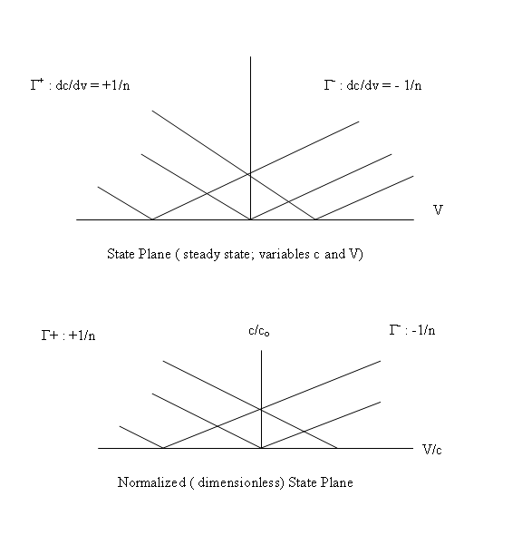
2.11 WAVE STABILITY
Compression waves are the rule in the physical
world. Density waves are always
compressive in nature, and all compression waves of finite amplitude grow
towards shocks. Only acoustic
compression waves ( i.e. infinitely low-amplitude compressions) are stable.
Finite rarefaction waves and rarefaction shocks are
impossible in material gases; only
infinitely low-amplitude rarefacttion waves can persist. ( however, see Sect.
6.11).
3. QUANTUM
PHYSICS
3.0 The standard
model of quantum physics is one of the most remarkable achievements of
science. It explains an enormous range
of nuclear an atomic phenomena to a very high degree of accuracy, and is
logically quite consistent. Yet, for all
its success, it has some serious deficiencies.
For example, while it is very successful in describing
many aspects of particle creations, annihilations and interactions, it still
has no predictive power to specify the values of the observed masses, and the
mass-ratios of the elementary particles – the experimentally determined values
of these masses must still be put into the theory by hand. Again, it requires the arbitrary introduction
of various fundamental constants, such as the fine structure constant of the
atom α, which are essential for its calculations, but for whose existence
or numerical value it has no explanation whatsoever. Again, quantum physics is still essentially
unrelated to classical mechanics, and although it can be related to
electromagnetic theory through quantum electrodynamics, this is so only for the
cases of the electron – the phenomena of the nucleus of the atom are as yet
still essentially unrelated to the rest of physical science in the standard
model of quantum theory. Yet again,
quantum physics has little relationship to relativity, gravitation and
cosmology.
3.1 COMPRESSIBILITY AND QUANTUM MECHANICS
All quantum phenomena are basically compressible
energy flow manifestations. The basic
energy form ( variously to be called a characteristic, enform, enray, ray, wave
pulse, wavelet, etc.) is the quantum wave function ψ which refers to a
single, compressible, enray pulse or wavelet.
More complex waves ( elementary particles, etc. ) are
built up from the linear enray ψ by superposition.
3.2 BASIC QUANTUM WAVE
The enray ψ is the linear, ‘characteristic’, or
‘ray’ solution, of the hyperbolic, linearised, approximate differential
equation called the classical wave equation ( Sect. 2.5.1; 2.6).
Ñ2ψ =
1/c2 ∂2ψ/∂t2
; ∂2ψ/∂x2
= 1/c2 ∂2ψ/∂t2
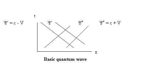
Therefore, the basic formula for the characteristic or
enray is as follows:
Ψ = c ± V
(1,2)
3.3 INTERACTING (NON-PARALLEL) QUANTUM WAVES
.. 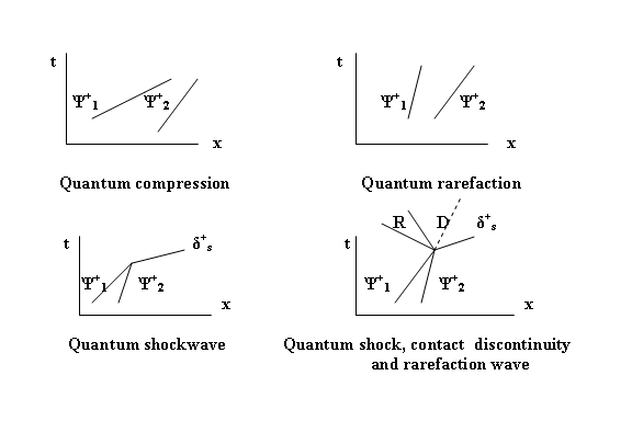
3.4 CURVED CHARACTERISTICS
In the general case, characteristics may be curved in
space-time, ( i.e. on the physical plane), indicating the presence of force and
acceleration.
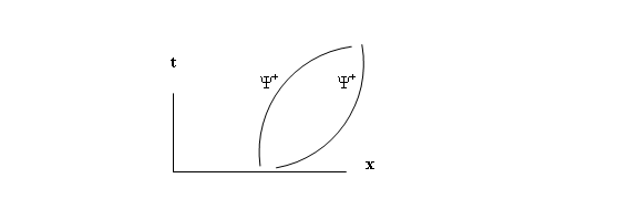
3.5 QUANTUM WAVE FUNCTION
ψ = c ±
V
(1,2)
Here, V is the relative velocity and may be set to
zero, making c = co in the ‘at rest’ coordinate system chosen. (cf.
Sects. 2.8; 5.2). For an energy flow, co is 3 x 10⁸m/s.
In general, ψ is complex, and we then have
Ψ = c ±
iV
(3)
3.5.1 NORMALISED QUANTUM WAVE FUNCTION
From (c/co)2 = 1 – 1/n (V/co)2, (Eq. 11, Sect.2.1), we have
ΨN = c/co + i V/co; ψ*N = c/co –
i V/co
(5)
For small V ,this reduces to ψN ≈ c/co.
The same wave speed ratio c/co gives all
the isentropic thermodynamic variable ratios
(Sect. 2.9). It also gives the Fitzgerald contraction factor of special
relativity ( Sect. 5.2.1).
3.5.2 THE (SPECIFIC) ENERGY OF THE WAVE FUNCTION
Eψ
= (c – iV)2 = (c + iV)2 – 2icV
(6)
Eψ*
= (c + iV)2 = (c2 –V2) + 2icV
(7)
For ‘mixed’ energies we would have no 2cV term:
(c + iV)(c –
iV) = c2 + V2 = [Eψ]2
(8)
(c+ V)(c – V) = c2 - V2
3.5.3 THE ‘EXTRA ENERGY’ TERM, 2CV
The term (c2 + V2) in (8) is the
familiar, elliptical ,steady state energy from the basic energy equation (
Sect. 2.1). The
‘extra energy’ term 2cV in (8) can be interpreted as being a transformation of
the coordinate axes c and V , by rotation through an angle θ.
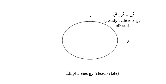
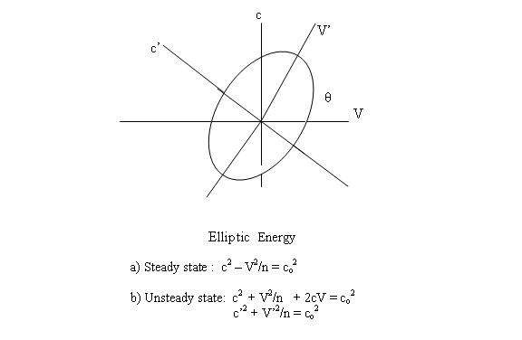
On the other hand, the energy term (c2 – V2)
in (7) is a theoretical oddity, namely a steady state, ‘hyperbolic energy’ with
no aparentg physical meaning. ( But, see Sect. 6.2.1). We may also note in
passing that, if the ‘extra enegy’ term 2cV is constant, then it, taken by
itself, has a hyperbolic interpretation, namely the form of an equilateral
hyperbola ( xy = const.)
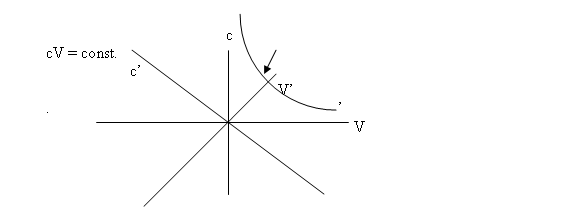
Hyperbolic energy:
a) Steady state: c2 – V2 = co2
; b) Unsteady : -2cV = co2
3.6 THE ‘EXTRA
ENERGY’ TERM (2CV) YIELDS THE FOLLOWING FUNDAMENTAL QUANTUM
RELATIONSHIPS:
A) PLANCK’S CONSTANT, h
For n = 1, if cV = constant energy for each set of
waves, then cV/υ = constant energy per cycle or pulse:
cV/υ
= h
cV =
hυ = hω/2π = ħω = ευ (9)
For the complex case,
cV/υ
= ħ/I = -iħ
(10)
B) DE BROGLIE WAVE/PARTICLE EQUATION
cV/υ
= h
But c/υ =
λ; V(m) = p (momentum), so
λp = h, or
p =
h/λ
(11)
C) LAGANGIAN FUNCTION, L
L =
2cV (see Sect. 2.3)
See also Sect. 4.7.3. for application to Hamilton’s
principle of Least Action for mechanical systems and to Fermat’s principle of
Least time for optical rays.
D) QUANTUM WAVE FUNCTION OPERATORS:
a)
HAMILTONIAN ENERGY
cV=
hυ = -ħω = ε
icV = -iħω
But
iω = ∂../∂t,
and so cV = h/I ∂../∂t = +iħ∂../∂t = Hop
which is the Hamiltonian energy operator.
( To ensure correct dimensions, it must be applied to
the normalized quantum function ψN).
b) MOMENTUM
cv = hυ =
+hω = ε
V = (1/c))ħω,
or (m)V = p = (m)(1/c)ħω
Multiplying by i, we have:
(m)iV = (m)(1/c) iħω
= (m)(1/c) ħ
∂../∂t
So, we have
(m) V = p = -(m)(1/c) iħ ∂../∂t
But,
I1/c) ∂../∂t
= ∂../∂x, and so
(m)V = p = -iħ∂../∂x = pop
(15)
which is the quantum wave operator, ( to ensure
correct dimensions, it must be applied to the normalized quantum function
ψN).
E) HEISENBERG UNCERTAINTY PRINCIPLE
cV =
hυ; cv/υ = h
λV = h
But x = Δx and V(m) = Δp, so
Δx .
Δp ≥ (m) h (16)
which is the Heisenberg uncertainty principle.
F) SUMMARY:
We have, therefore, related
all the above fundamental quantum relationships to a single energy term 2cV.
We have, in effect, quantized the various energy
‘fields’ represented by 2cV/n for various values of n, by equating them to the
‘time-like’ condition set by the frequency υ in the quantum equation
hυ = 2cV/n.
(Note that these equations are for ‘specific’ energy,
that is, for unit mass flow. For a
definite particle, the numerical value of the mass is to be inserted; the
dimensions of the equations are not thereby changed, since in our system, mass
(m) is dimensionless. Thus for the photon, we have hυ = me cV,
where me is the relativistic mass of the electron. In terms of the
momentum, we have
hυ = cp,
which is the de Broglie equation (Eq.11).
3.7 QUANTUM WAVE/PARTICLE EQUATIONS
The quantum operators for momentum and Hamiltonian
energy in Sect. 3.6 D then lead to the various standard quantum wave equations
for the elementary particles:
3.7.1 SCHRODINGER EQUATION
For a non-relativistic, spinless particle we have
-ħ2/2m
Ñ2ψ = iħ Ñψ/∂t (17)
3.7.2 DIRAC EQUATION
Eψ + c(α . p )ψ + moco2βψ = 0
Or,
iħ∂ψ/∂t
= iħcα . Ñψ + moc2βψ = 0
(18)
where α12 = α22
= α32 ; β = 1.
3.7.3 KLEIN-GORDON EQUATION
For a relativistic, but spinless particle, we have
Ñ2ψ =
1/c2 ∂2ψ/∂t2 [moc/h]2
ψ
19)
3.7.4 WEYL
EQUATION (NEUTRINO)
For a massless, spin one-half particle we have
Iħ ∂ψ/∂t = iħ cα . Ñψ
Or,
Iħ ∂ψ/
t = (σ . p) ψ
(20)
3.8 QUANTUM STATE FUNCTIONS
The quantum state functions are the normalized form of
the state variables, namely c/co and V/co. The state
plane characteristics Γ± (see Sect. 2.10 b) are:
Γ+
: dc/dV = +1/n; Γ- :
dc/dV = -1/n
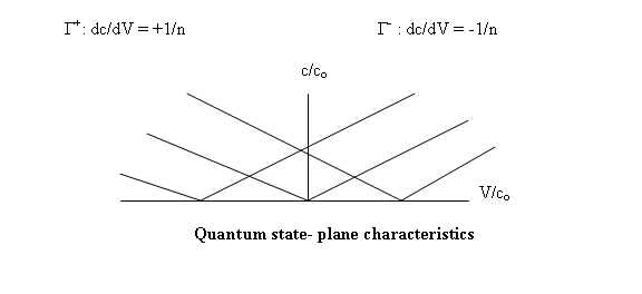
The isentropic ratios can be obtained from c/co,
just as in Sect. 2.9.
3.9 THE ORIGIN OF MATTER: ENERGY COMPRESSIBILITY
All elementary particles of matter (with the possible exception of the neutrino) are condensed
energy forms. The forms are given in terms of a simple, integral number n (
n = degrees of freedom of the compressible energy flow):
A. BARYONS AND HEAVY MESONS
mb/mq
= Vmax/c* = [n+1]1/2
(21)
mb is the mass of any baryon particle, mq
is a quark mass, Vmax = co n1/2 is the escape
speed to a vacuum; that is, it is the maximum possible relative flow velocity
in an energy flow for a given value of n, the number of degrees of freedom of
the energy form, (see Sect. 2.7 for compressible flow velocity ratios). This is a non-isentropic relationship, and it
corresponds physically to the maximum possible strong shock. (See Sects.
2.5.3.3 and 3.13).
Experimental verification for thisw baryon mass ratio
formula is given in Table 3.9.1A below.
B. LEPTONS, PION AND KAON
mL/me-
=
k/α2 = [(n+2)/n]/α2 = {(n+2)/n] x
137
(22)
where α = 1/11.703 is the fine structure
constant, and k is the adiabatic exponent or ratio of specific heats, k = cp/cv
= [(n+2)/n]. (See Sects. 3.10; 3.11). Because of the presence of k, this
formula for the mass of the leptons is a thermodynamic and quasi-isentropic
one.
The leptons are formed via the weak shock option 9 See
Sects. 2.5.3.3 and 3.13).
The experimental verification for the lepton mass
ratio formula is given in Table 3.9.1B below.
3.9.1 EXPERIMENTAL VERIFICATION OF MASS-RATIO
EQUATIONS (21) AND (22)
A) BARYONS AND HEAVY MESONS
--------------------------------------------------------------------------------------------
n n +1 [n+1]1/2 Particle Mass (mb) Ratio to
(MeV) quark mass
0 1 1 quark (ud) 310 MeV 1
(s) 505
1
2 3 1.73 eta (η) 548.8 1.73
3
4
5 6 2.45 rho (ρ) 776 2.45
6
7
8 9 3 proton (p) 938.28 3.03
(1)
neutron
(n) 939.57 3.03
Λ
(uds) 1115.6 2.97
(2)
Ξo
(uss) 1314.19 2.99
(3)
9 10 3.16 Σ+ (uus) 1189.36 3.17
(2)
10 11 3.32 Ω- (sss)
1672.2 3.31
(4)
Note: Average quark mass is 310 MeV; (2) Average quark
mass is (u + d+ s)/3 = 375 MeV (B)
Average quark mass is (u+s+s)/3 = 440 MeV; (4) Average quark mass is 505 Mev.
Therefore, Equation 21 is verified.
B) LEPTONS, PION AND KAON
N k =
(n+2)/n Particle Mass Ratio Ratio
(MeV) to x 1/137
Electron
1/3
7 Kaon K± 493.67 966.32 7.05
2
2 Pion π± 139.57 273.15 1.99
4
1.5 Muon μ 105.66 206.77 1.51
-
- Electron 0.511 1
Clearly, k ≈ ml/me
(1/137), verifying Equation (22).
The lepton/meson mas
s formula (22) for a weak shock condensation also has
a thermodynamic interpretation:
mL/me- = cp/cv
1/α2
(23)
α2 = ml/me-
cp/cv [ ΔT/ΔT] = (ΔQL+)p/(ΔQe)
= 1/137
(24)
3.9.2 SUMMARY
Equations 21 and 22 give, for the first time, an
experimentally verified explanation for
the origin of matter, and for the observed ratios for the masses of the elementary
particles of matter. The principle of the compressibility of energy flow,
therefore, underlines all material particles and the whole material universe.
\The text of Summary of a Universal Physics has been revised to this point as of
Sept. 29/03. The remaining sections which were composed in 1992 and previous
years will be successively reviewed and revised as necessary in future Website
Updates.
3.10 ENTROPY AND THE MASS RATIOS
If the entropy is taken to a binary logarithmic base,
that is, if
S = log2
n
(25)
Where n =1,2,3,….., and if these values for S are then
compared with the values of [n+1]1/2, which give the baryon and heavy meson mass ratios from Eqn. (21), we
see that there is only one value for n which gives the same value to S as
computed and for [n+1+]1/2. This is n = 8, the value for n for the
proton (Sect. 3.9.1). We then have
[8+1]1/2
= 91/2 = 3 = mb/mq
log2
8 = 3 = S(n=8)
The proton is the most stable elementary particle of
nature, whereas all other baryons have fleeting lifetimes. It appears that n = 8 is a unique value,
since it is only for this value that the binary logarithmic formula for
computing the entropy gives a value
which equals tke necessary baryon mass condensation ratio [n+1]1/2.
This unique equality may underlie the observed stability of the proton.
aryon particles.
3.11 ENTROPY AND THE FINE STRUCTURE CONSTANT
The fine structure constant of the atom α =
-1/11.706 is the fundamental electron/photon interaction, or coupling constant. Its square is approximately 1/137,
and this number determines the probability of emission and absorption of
photons in electromagnetic interactions.
We recall that entropy is given by S = ln n, dS =
dn/n/ and ΔS = Δn/n, n being a large number. However, at the elementary particle level, n, the number of degrees of
freedom of the compressible energy flow, is small; typically n equals 1 to 8 (see Sect. 3.9.1).
This would suggest that entropy change here is given by
Δs =
Δn/n
For example by ½ -1/3, 1/3 -1/4, and so on, the value
of Δn being unity.
However, in compressible flow, the entropy change
ΔS accompanying any non-isentropic process, such as a shock transition or
a contact discontinuity, would be given by a formula such as the following one:
Sy – Sx = ΔS = ln(1+P) – k
ln(1 +((k + 1)/2k))P) + k ln(21+ ((k-1)/2k))P)
Where k is cp/cv and P is the
shock strength expressed in terms of the pressure rise across the shock py/px and is given by
P = py/px
– 1
If the shock is very weak ( and this would correspond
to electromagnetic interactions controlled by 1/137), then the following
approximation applies:
Δs/R = [Sy
– Sx] = 1/12 (k-1)/k2
p3 – 1/8 (k+1)/k2
p4 + …..
Now the mean value of the first term factor which
multiplies p3 , computed over a range of values of k corresponding
to n varying from 1 to7 is 1/11.6907;
this is within about one part in a thousand of the accepted value for
α, the fine structure constant.
It is even more interesting that, if we suppose that
the formation of proton plus electron involves an ‘all-possible-paths’ entropy,
and then compute this for n = 8 (proton) and n = 9 ( i.e. (n +1), we get
ΔS = [ln
8! + ln 9!)/2 = - 1/11.703215 ≈ α (28)
The experimental value for α is about
-1/11.706244, so that this extraordinarily simple calculation gives a
theoretical computed value for α to within 3 parts in 104.
Again, various shock formulae also give values which
are quite close to the experimental value for α when n in the range
indicated. Further refinement of this new approach to a derivation of the fine
structure constant α on physical compressibility grounds in the stanounds
is left to specialists in quantum perturbation theory and charge
renormalization.
It should also be noted here that the supposition of
the involvement of shock transitions in particle structure also imposes a
physical limitation to the close approach of electrons to one another, as is
actually required on theoretical grounds in the standard model of quantum
electrodynamics in order to avoid the problem of infinities in charge
renormalization procedures.
On the state plane, we see that a change in entropy
ΔS plots as a rotation of the state plane characteristic Γ through an
angle θ as the value of n changes (Sect. 3.8).
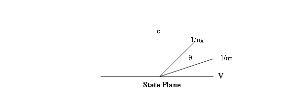
3.12 QUANTUM INTERACTIONS AND ELEMENTARY PARTICLE
GENERATION: GRAPHICAL DEPICTION
Two interacting enrays or quantum functions of the
same family (ψ+1,2) form a finite-amplitude, third
wave which immediately grows to form a shock (δ+s),
( see Sect. 2.10).
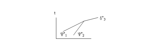
Two interacting shocks (δ+1,2)
produce a third shock (See Sect. 2.9.1).
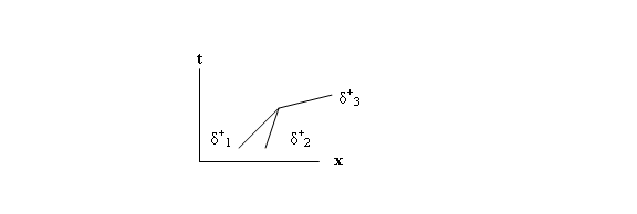
If the interacting shocks are quarks (q+1,2)
the resulting elementary particle formed is a roton or neutron (p,n) .
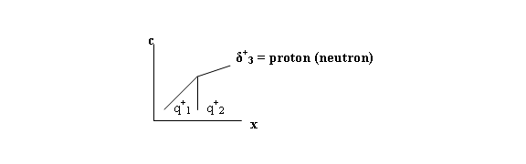
These interactions are in order of increasing
strength.
Continuity requirements and entropy considerations
require that the proton generation process also produces a contact
discontinuity (D) which is the physical basis for the electron (e-)
Sect. 4.1.1), as well as a balancing, simple rarefaction wave R which is the
source of the (anti-) neutrino (ν) Sect. 2.10).
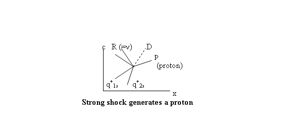
The u,d quarks combine two-by-two (q+1,2)
in the above model to form the proton.
This means that the entropy changes involved in the process have a binary
logarithmic basis. (Sect. 3.11.1).
The mass ratios for the generating particle and the
generated particle are in the ratio of the shock condensation densities. For
the baryons, this is
ρ2/ρ1
= [n+1]1/2
(21)
The leptons and electron form via the weak shock
option.
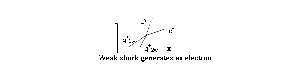
3.13 RADIOACTIVE DECAY
Baryon particles form via the strong shock condensation
(Sect. 3.9;2.5.3.3), with the condensation ratio typically being specified by
the parameter [n+1+]1/2 in (21).
Baryon particles decay via the weak shock otin (Sect.
3.9; 2.5.3.3);
The weak shock typically occurs when the back, or
downstream pressure is low. The
continual formation, reflection, reformation process for particle
stabilization, plus the two shock options underlie the observed probabilistic
basic for radioactive isotopic decay of b 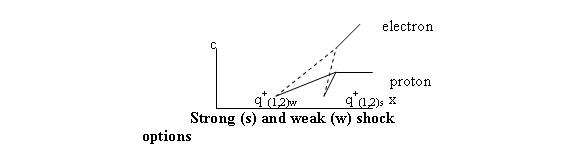
3.14 SPIN, REFLECTION, PARTICLE CONFINEMENT AND
SPINORS
The interaction of two enrays produces the elementary
baryon particles by shock condensation ( Sect. 3.9). Total internal reflection
of the shock regenerates the enray pair, and the process is then endlessly
repeated unless and until the weak shock option is chosen, whereupon
radioactive decay occurs.
The particle stabilizes by confinement under total
internal reflections of the 2-enray/shock ensemble at the refractive index
interface between the particle and the surrounding vacuum, (see sect. 4.7.1).
Each flow reflection generates a ‘flip’ or spin of
180° (spin ½) for a coupled , 2-enray spinor, and a 360° rotation or spin 1,
for a 3-enray set. (see Sectd. 4.5.5).
Each shock reformation (particle formation) entails
the choice of either the strong shock option ( i.e. particle stabilization and
continuity of existence), or the weak shock option (particle dissolution via
radioactive decay). (cf. Sect 2.5.3.3).
The spin is related to the number of enrays
interacting according to the usual formula
N = 2S + 1
The behavior of sets of coupled interacting enrays is
described mathematically by the spinor calculus.
The details of confinement and spin must be left for
the appropriate specialists to evaluate.
3.15 QUANTUM CREATION AND ANNIHILATION OPERATORS
In the standard model of quantum theory, these have
the following form:
A* |n> =
(n+1)1/2|n+1>
The new theory equates the [n+1]1/2 term to
the maximum possible compressible flow condensation ratio (Sect. 3.9, Eq.
(21)), which specifies the masses of the baryons and heavy mesons.
In our compressible system, we designate each separate
energy ‘field’ which is to be subjected to the ‘second quantization’ so as to
generate an elementary particle, by choosing values for n, the number of
degrees of freedom of the energy transformation. Since the quantization also involves the
expression hν, (Sect. 3.6), where ν is the frequency kit is a
‘time-like’ quantization. ( For a
“space-like” quantization see Sect. 6.2).
3.16 THE COLLAPSE OF THE WAVE FUNCTION PROBLEM
The physical act of measurement or detection of the
quantum wave pulse converts it to a shock wave, and this physical
transformation is involved in the so-called ‘collapse of the wave function’
problem. (See also sects. 6.3 and 6.10).
The probabilities involved in the self-interference of
the wave function ( for example in the two-slit interference experiment) are
also associated with the extra energy term or wave perturbation term 2cV/n.
3.17 NATURE OF THE QUANTUM WAVE FUNCTION
The position of the new theory as to the nature of the
quantum wave function is one of scientific realism. That is, the quantum wave function represents
a basic physical entity of compressible energy flow, one which, however,
is grasped, not imaginatively, nor symbolically, but rather in the
intelligibility of its correlation with the scientific formalism of compressible
flow theory.
3.18 FEYNMAN DIAGRAMS AND VIRTUAL PARTICLES
The Feynman diagram ( and space-time relativity
effects see Chapter 5) can be interpreted as depictions of compressibility
effects in the physical plane, which is the x,t or space-time diagram.
The intermittent aspect of the existence of the
elementary particles (Sect. 3.14) is closely related to the virtual particle
concept of standard quantum physics.
3.19 DIRAC DELTA FUNCTION
The mathematical delta function δ corresponds to
a wave pulse discontinuity, such as a shock wave in the compressibility
formalism.
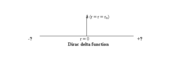
4.
ELECTROMAGNETISM
4.1 THE PHYSICAL BASIS OF ELECTRIC CHARGE
4.1.1 CHARGE AND VORTEX MOTION
As already seen in the new theory (Sect. 3.9), matter
has the nature of a localized condensation in energy density, with its
magnitude being given for the baryons and heavy mesons by the equation
mb/mq
= [n+1]1/2
and with the condensation taking place by the strong
shock.
For the leptons, pion and kaon, he condensation is
given by
ML/me-
= k/α2 = α2
cp/cv = (n+2)/n (1/α2)
With the condensation process taking place by the weak
shock.
Physically, the condensation takes place in either shock
option at the intersection of two enrays in an energy flow (Mach lines, shocks,
quarks, etc.). Furthermore, since the tgo interacting enrays must be of unequal
strength ( i.e. having unequal slopes on the space-time diagram), then a third
phenomena – a contact discontinuity line D
-emerges.
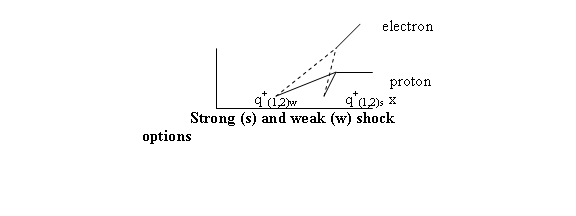
In standard quantum mechanics, electric charge has
some formal resemblance to angular momentum, which, however, is considered to
be only a mathematical coincidence; in the new theory, electric charge has a
physical origin in vortex motion.
4.1.2 VORTICITY AT A CONTACT DISCONINUITY
In the case of a compressible flow interaction, we
have
2ω = -∂V/∂N -(1/ρV) ∂p/∂N
(1)
where N is a space direction normal to the flow
streamlines, ω is the rotation and p is the pressure.
In the case of two intersecting pressure pulses
(waves) we have
2ω =
-11/V [ T ∂S/∂N - ∂ho/∂N ]
(2)
ho is the stagnation enthalpy ( h = U +
pv), T is the temperature. The vorticity
then depends on the rate of change of entropy and stagnation enthalpy normal to
the flow directions.
4.1.3 ENTROPY AND CHARGE
In quantum theory, the charge e-, has the
nature of an electromagnetic force coupling constant (e- = ge). The square of the charge constant is equal to
the square of the fine structure constant of the atom:
e-2
= ge2 = e2/ћc = α2 = [1/11.7]2
= 1/137
(3)
But, (Sect. 3.11), the fine structure constant α is
also an entropy, and we have , when n := 8
and (n + 1) = 9 :
ΔS = ( ln
8! + ln 9!)/2 = α ≈ -[ 1/11.7]
3a)
The entropy change across a contact discontinuity
resulting from the interactin of tdwo unequal generating sshocks, or unequal
characteristics, (ψ+1,2), is also a measure of
electgric charge e-.
4.1.4 ENTROPY AND PRESSURE RATIO
ΔS = S2
–S1 = -R ln(p02/p01)
(4)
4.1.5 COMPRESSIBLE POTENTIAL VORTEX (CPV)
Vr =
const.
(5a)
R*/rmin
= [n+1]1/2
(5b)
Vmax
= n1/2 co
(5c)
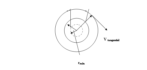
4.1.5.1 COMPTON WAVE LENGTH λc
In the compressible potentiall votex (CPV), we have
λ c
= n1/2 rmin ; rmin
= λc/n1/2
(6)
r* = λc
[ (n+1)/n]1/2
(7)
rBohr
= λ? (1/α2)
(8)
4.1.6 ELECTRON VORTEX PRESSURE
c/co
= (p/po)1/(n+2) = [ 1 – 1/n{V/co}2]1/2
(9)
4.1.7 MODEL OF THE HYDROGEN ATOM
We have two vortex flows and their combinations:
A) THE ROTATIONAL VORTEX (RV)
V T/r
= const; V T = rω =
(Г/2π)r
(14)?
At the rim of the vortex: V T = Vmax = n1/2 co.
B) THE COMPRESSIBLE POTENTIAL VORTEX (CPV)
VT
r = const.; rmin = λc/ n1/2
(see Sect. 4.1.5).
C) THE HYDROGEN ATOM: (NUCLEUS + ELECTRON)
Various combinations of A and B above may be
considered for a model of the atom. We
present here a double CPV model, with the nucleus being a CPV of dimensions
approximately 10-15 m , surrounding an electron CPV with a radius
which is approximately the Bohr radius ( 10-10 m).
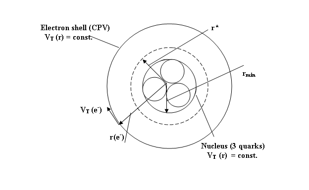
4.1.8 de BROGLIE WAVELENGTH, λde B
λde
B = 2πλc[c/V]
(15)?
Wgere c/V is the invcerse Mach number (1/M) of the
energiy flow.
Λc
= [λde B/2π]
V/c
(16)?
4.2 ELECTROSTATIC FIELD
A stationary charge is surrounded by an electrostatic
field, which, on the new theory, consists of a field of virtual photons
emanating from the CPV of the electron.
The virtual photons are Mach line characteristics of the flow, emitted
symmetrically into space in the near field surrounding the electron. The characteristics terminate on a sink (
i.e. on another charge) confined to the near field, that is to within one
wavelength. These curved characteristics
are identified with the electromagnetic field lines. The curvature of the
characteristics in space-time reveals the existence of force in a compressible
flow (Sect. 3.4).
4.3 MAGNETISM: THE COMPRESSED VIRTUAL PHOTON
FIELD OF A MOVING CHARGE
The electric field of a moving charge is compressed in
the direction of the motion: a
solenoidal magnetic field then emerges
as a relatsivity ( i.e. compressibility ) effect (Sect. 5.2).
4.4 ELECTROMAGNETIC RADIATION
A stationary charge has a symmetrical, virtual photon
field; a uniformly moving charge has a
compressed virtual photon field which generates a solenoidal magnetic field; an
accelerated charge represents a discontinuity ( or pulse) in virtual photon
concentration. When the charge is
accelerated, this concentrative gradient in the virtual photon field detaches
itself from the charge or charges, (source or sink) and travels outwards as a
set of photons which are no longer virtual but real. Maxwell’s classical equations for the
electromagnetic field follow naturally (Sect. 4.5.1).
4.5 THE PHOTON STRUCTURE
When two characteristics interact ( sect. 2.19), for
example in so-called corner flow, they encounter a structural flow ambiguity which
is resolved by the formation of a shock.
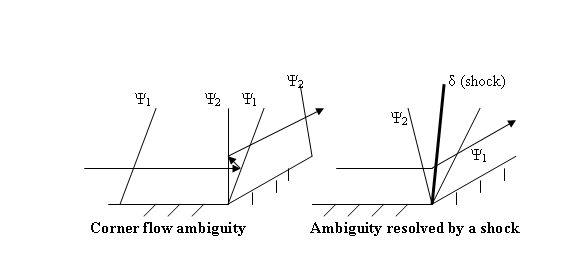
When three characteristics interact, they for a cusp/envelope
region in the flow and the three characteristics then meet at a point/ There is
again an ambiguity in the flow.
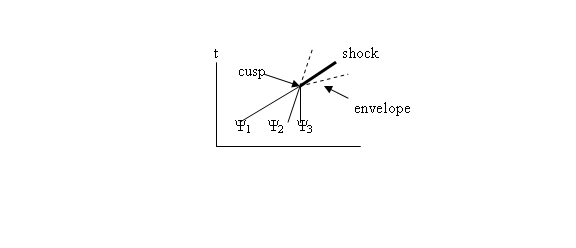
The ambiguity at the crossing point of the three
characteristics is resolved by a 360°rotation or spin, and the transverse,
rotating vector constitutes the photon.
4.5.1 CUSP VECTOR FIELD (NON-CO-PLANAR)
Three, non-coplanar vectors combine to give
Ψ1 x (ψ2 + ψ3)
= (ψ1 . ψ3ψ2) – (ψ1
. ψ2ψ3)
Which is the curl of a vector field, B = curl A: so that
Curl B = curl curl A = Ñ( Ñ x A) = Ñ×ÑA - ÑÑA
= grad div A - Ñ2A
This connects the three characteristics of the
compressible flow ( i.e. three non-coplanar vectors) in the new theory with
Maxwell’s equations:
Ñ X E = 1/c ∂B/∂t div E = D
(17)
Ñ X B = 1/c ∂E/∂t div B = 0
(17)
4.5.2 PHOTON ENERGY
ε = hν = cV
(18)
h = (c/ν)V = λV
But, for the photon, V = co, and so
H = λ(m)V
= λp
which is the de Broglie equation for the photon.
4.5.3 PHOTON SPEED
In the energy equation for 1-dimensionl motion, n
equals unity, and we have
c2
= co2 – V2 , and so
Vmax
= n1/2 co = co
The photon speed Vγ is, therefore, the
escape velocity to a vacuum Vmax
which equals co (= 3 x 10⁸ m/s).
In free space the photon speed corresponds to Vi, the
particle speed of the flow. In matter, or in interactions with matter, the
photon speed corresponds to V, the local relative flow speed (Sect. 4.7.1).
4.5.4 RELATIVISTIC FORM
The above 3-vector description of the photon equation
I classical Maxwellian form for a sokple cokmpressible flow an be cast in
relativistic form by introducing the 4-vector potential Aμ
Aμ
= A(x,y,z,φ)
Where φ is the velocity potential.
4.5.5 PHOTON SPIN
Spin involves an analysis of the streamline ambiguity
which arises from some flow reflections, the relationship between the
streamline directions and the characteristic direction requires that a
2-cmponent flow undergoes a 180° ‘flip’ or spin upon reflection of the flow
(Sect. 3.14).
A 3-component flow, such as for the photon, requires a 360° rotation or
spin upon reflection. This agrees with the usual spin equation, where N is the
number of flow components:
2S + 1 = N
For example, if N = 3, we have S = 1, and this
corresponds to the photon spin.
4.6 THE MICHELSON-MORLEY EXPERIMENT
In compressible flow theory, the flow velocity V in
the energy equation
c2
= co2 – V2/n
is always purely relative, and this same equation also
yields the Fitzgerald contraction factor (Sect. 5.2.1), ( provided that n in
the energy equation is equal to unity, for example for 1-dimensional motions):
c/co
= [ 1 – (V/co)2]1/2
Thus, since only relative velocity V enters, there are
no absolute motions involved which can effect the system; the observed null
result of the Michelson-Morley experiment is therefore to he expected as a
simple consequence of the existence of compressibility in the energy flow. Note also that in compressible flow theory,
the M/M experiment is also seen as an isentropic process.
4.7 SOME OPTICAL EFFECTS AND THE FIZEAU
EFFECT
4.7.1 THE REFRACTIVE INDEX N
The standard definition of the refractive index N is
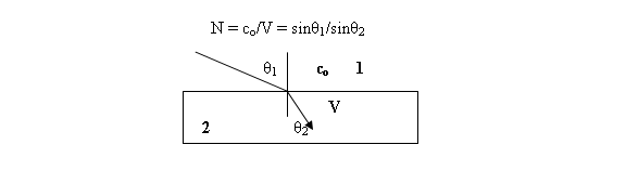
So that N is the ratio of the speed of light in vacuum
to the speed in some optical medium.
To express N physically as a compressibility
phenomenon, we proceed as follows:
c2
= co2 –V2/n
from which we have the following relationships
c = [co2
– V2/n]1/2 c/co = [1 – 1/n (V/co)2
]1/2
V = [nco2
– nc2]1/2
V/co = [1 – (c/co)2]1/2
And, for V = c = c* , we have c* = V*
c*/co
= [n/(n + 1)]1/2
Finally, we put
N≡ Vo/Vi
Where Vo is the speed of photons in vacuum,
and Vi is the speed of photons in the optical medium.. We therefore
have expressed N in terms of two compressible flow velocities.
Note that the photon speed, or speed of light, is not
identified with the wave speeds, c or co, but with the relative flow
velocity V instead. However, the energy of the photon involves the wave speed c
and the relative flow velocity V ( Sect. 3.6).
Now, the ratio of the two speeds of flow Vo/Vi
has the identical form of the left hand side of the Prandtl equation for the flow
velocity transformation across a normal shock front, namely
Vo/Vi
= c*2 / Vo2
And, if Vo = co, then also
Vo/Vi
= c*2/co2 = (n+1)/n
But we have
set Vo/Vi equal to the refractive index N and so we also
have
N = Vo/Vi
= (n+1)/n
relating the refractive indeed N to the compressible
flow parameter n.
Thus the reduction in the speed of light in an optical
medium having refractive index N with respect to the speed of light in space is
explainable physically as a reduction in an upstream compressible flow velocity
Vo relative to a downstream flow velocity Vi across a
normal shock front occurring in a compressible energy flow, these two flow
velocities being identified with the photon velocities outside and inside the
optical medium.
The relationship N = (n+1)/n Is shown in the following
table for integral vales of n:
Degrees of
Freedom n versus
Refractive
Index N
n N
1 2
2 1.5
3 1.33
∞ 1
We note that the predicted range of the values for N,
corresponding to simple vales of n ranging from 1-dimensionlal flow to
3-dimensional flow, covers the known values for N for over 99% of all optical
media where N lies between 4/3 and 2.
The convention of making N for free space equal to unity also
corresponds to a value for n of infinity, and this is the value for a pure
field. The electromagnetic shock
hypothesis thus yields a prediction for the value of N corresponding to
observed data. We conclude that N is in
fact, physically based in a normal shock transition across the interface
between an optical medium and free space.
We reiterate that the speed of light Vo in
space ( = 3 x 10¹⁰ m/s) is a flow speed and not co, the
free –space wave speed; the speed of light Vi in the medium is again
the flow speed and not the wave speed ci . The wave/particle nature of the photon is,
however, not affected by this since the photon energy is given by the product
of c the wave speed and V the particle speed ( ε = hν = 2cV) (Sect.
3.6)) .
Refractive indices intermediate in value between the
values in the table should be explainable in terms of flows of mixed
dimensionality. Media with N less than 1
or greater than 2 would involve either fractional degrees of flow freedom or
flows of dimensionality higher than three.
In interpreting the mechanism further, it is worth
noting tht the interface between an optical medium and space is, on the atomic
scale, not ‘flat’, and so a transition interfacial state should be considered
in any detailed or rigorous modeling.
4.7.2 THE FIZEAU EFFECT
The above derivation of N refers to stationary optical
media. When the optical medium moves,
(e.g. flowing water), then the experimentally observed fractional addition of
velocity to the speed of light caused by the speed of the medium Vm
is usually explained as a relativity effect which can be calculated from the
Lorentz/Einstein velocity-addition formula for transformation of velocities
between coordinate systems in uniform relative motion:
V = [co/N
+ Vm] / [ 1 + (coVm/N)/co2]
Which, when expanded as a power series in V/co,
gives
co/N
+ Vm[ 1 – 1/N2]
where the bracketed factor is the Fresnel drag
coefficient.
This drag coefficient, however, is an isentropic flow
factor derived from the compressible energy equation, since
(c/co)2
= 1 – 1/n (V/co)2
If n = 1 (1-dimensional flow) then (V/co)2
= 1/N2, so that
Fresnel/Einstein drag coefficient.
This raises a logical problem, because, if the index
of refraction N is to be explained by a shock mechanism for a stationary flow,
then this is a non-isentropic process.
Why then is the addition-of-velocity drag formula for a moving medium
explained by an isentropic flow formula?
In the past, it has been proposed that there are
observable discrepancies in the experimental data, which in fact point to a failure of the isentropic
Fresnel/Einstein drag formula for moving media, and which argue instead for a
shock transition formula for moving media as being the correct one. Another possible explanation lies in the
well-known fact that, for weak shocks the differences between the
non-isentropic or shock formula and the purely isentropic formulae show up only
in terms higher than second order in the shock strength. Shocks involved in compressible theory for
values of N between 4/3 and 2 would be relatively weak, and so the numerical
differences in the predictions of the two mechanisms - isentropic and
non-isentropic- would be small.
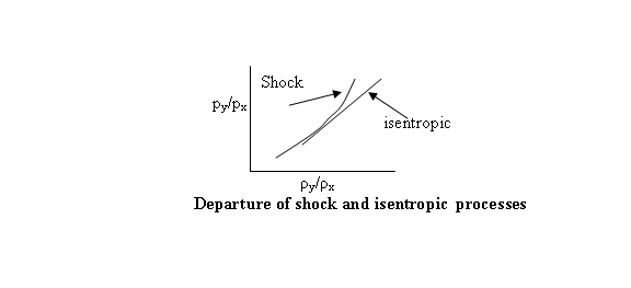
It is pointed out that the Fizeau effect, unlike the
Michelson and Morley effect, is first
order in (V/c) and is readily observable; it merits further analysis,
and the experimental discrepancies should be carefully examined in the light of
the various possible mechanisms involved.
4.7.3 FERMAT’S LEAST TIME PRIINCIPLE FOR
OPTICAL RAYS
In classical mechanics, Hamilton’s principle of Least
Action applies widely. It is expressed
as
δò L dt = o
where L is the Lagrangian function.
But, in our new theory L = cV (Sect. 3.6C), and so
δò L dt = δò Vc dt = δò V ds =0
where ds is the invariant metric interval. In such systems, for example simple harmonic
motions, L varies constantly or periodically and so, therefore, do c and V.
But, in a homogeneous optical medium, c and V are
constant, and so we must put
δò L dt = δò cv dt = δò dt = 0
which is Fermat’s principle of a least time path for
optical rays.
Both Hamilton’s principle and Fermat’s can be derived
from the cV term in the unsteady flow compressible energy equation; if cV
varies, Hamilton’s least action result, if cV is constant, Fermat’s least time
applies.
4.8 THE SAGNAC EFFECT
In this interesting effect, an interferometer is
rotated and a fringe shift δ is then observed which is given by
Δ =
(4Ώ A)/λoco)
(28)
Where A is the area enclosed by the light path, Ώ
is the angular rate of rotation, λo and co are free
space values.
4.9 DE BROGLIE EQUATION
In the de Broglie equation λ = h/p = h/mV, upon setting ε = hν = (m) c2. we
obtain the equation
upvg
= co2
This derivation requires that the phase velocity up
should exceed co when vg is small.
The new theory ( Sect. 3.6B) has, however, put
ε
= cV
instead of ε = (m) c2.
From the unsteady state energy equation we get .
c2
= co2 – V2/n – 2cV/n, or
cV =
n[co2/2 – c2/2 –V2/2]
instead of upvg = co2.
The supercritical phase speeds which emerge from the
customary de Broglie derivation are avoided.
Note that cV emerges as a :sum of kinetic energy terms in co,
c and V.
4.10 THE PERIODIC TABLE
We have seen (Sects. 3.6B; 4.1.5.1; 4.1.8) that
( de Broglie wavelength):
λde B =
h/m/λ
(Compton wavelength):
λc = h/mc
so that λc/λde B = V/c
It is interesting that, if we now set
N λde
B = 2π re
(29)
We have
λde
B = (2π/N) re
(29a)
where N is a quantum number equal to 1,2,3….2π,
and re is an electron radius.
E valuating (2π/N) we get the following table:
N (2π/N) Electron
Shell
1 0.15915 K
2 0.31831 L
3 0.47746 M
4 0.63682 N
5 0.79577 O
6 0.95493 P
2π 1.00000 Q
We see that there are only seven possible
configurations available from Equation 29, if N is a positive integral quantum
number and re ≤ λde B.
This, and Eq. 29 are, of course, just the Bohr model
of the atom, except that the model has now been related to a compressible
(vortex) flow.
The full quantum theory of the atom requires the
Schrodinger equation ( Sect. 3.7.1), which has its compressibility basis in the
quantum operators for momentum and position as given in Sect. 3.6D.
5. RELATIVITY:
A COMPRESSIBILITY EFFECT
5.1 GALILEAN RELATIVITY
Communication signals are instantaneous (c = ∞
). Transformations are as follows:
l = l′ y = y′ t = t′ V′ = V1 + V2
z = z ′
x = x′ +
vt
5.2 SPECIAL RELATIVITY (Relativity of uniform motion)
Signals travel at a finite speed (c ‹ ∞ ), that
is, at the speed of light (3 x 10⁸ m/s) in free space.
The present theory identifies a finite speed of light
as a physically-based compressibility effect.
The photon speed is now explained as a flow velocity.
The free space speed is Vγ = 3 x 10 m/s. From the basic energy equation
c2
= co2 – V2/n
(1)
we see that V can only equal co if n = 1
and c = 0; this is the condition where Vγ = Vmax the
escape speed to vacuum.
The wave speed c is a local variable determined by V
and vice versa. The wave/particle nature
of the photon is evidenced in the new theory since the photon energy is
Ε =
hν = 2cV
So that it depends on both a wave speed c and a
particle of flow speed V. (Sect. 3.6).
If an arbitrary choice is then made to assume an
inertial coordinate system, namely one ‘at rest’, then the wave speed in free
space co (numerically equal to the speed of light Vγ
in free space) becomes equal to the free space speed of light relative to the
inertial system, and the variable wave speed c becomes transferred from the
inertial system to any other system moving at relative speed V. The famous postulate of the ‘constancy of the
speed of light in vacuum for all inertial observers’ has its roots in this
essentially arbitrary choice in the compressible energy equation.
5.2.1 THE FITZGERALD CONTRACTION FACTOR
This follows from the steady state energy equation (1)
c2
= co2 – (1/n) V2
(1)
where, for 1-dimensional flow where n = 1, we have
c2
= co2 – V2, and
c/c0
= [1 – (V/co)2]1/2 (2)
which is the Fitzgerald contraction factor, and which
is now seen being a compressibility ratio of wave speeds.
5.2.2 THE LORENTZ TRANSFORMATIONS
These now become a series of simple, kinematic, compressibility
ratios, all equal to the wave speed
ratio c/co, as follows:
c/co
= l′/l = dt′/dt = dτ/dt = x′/(x – vt) = t′/(t
–(vx)/co2) = W/Wo = Eo/E = mo/m
= Fo/F =
= λ/λ′ = ν/ν′ = p/po = T/To
(3)
where τ is the
proper time, W is work, E is energy, m is mass, F is force, λ is wavelength, ν is
frequency, p is momentum, T is
temperature.
Since c/co is also the fundamental
isentropic ratio, giving all the thermodynamic ratio values for pressure,
density and temperature , (see Sect. 2.9), the new theory now relates the
Lorentz transformations to these thermodynamic ratios, as well as to quantum
physics via the quantum state variables, c/co and V/co
(Sect. 3.8).
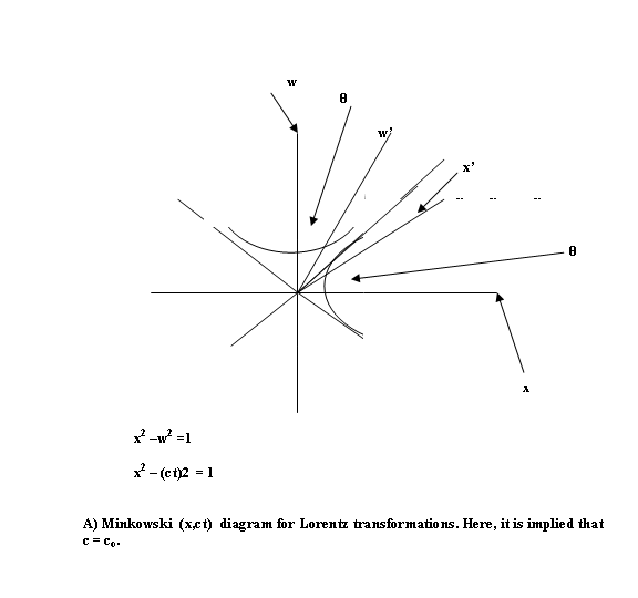
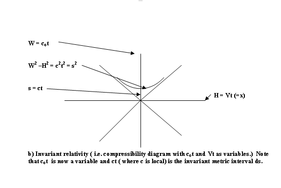
In (b) above the variables cot and Vt are
numerically identical to Minkowski’s c and x, but they are conceptually very different;
they are now physically-based, compressibility quantities involving the quantum
state variables.
The metric interval is
ds = c dt
(4)
where c is now the local
wave speed calculated from the energy equation (1), and dt is the local time
differential.
We derive the metric interval ds from the energy
equation as follows ( for n = 1): In the energy equation (1) co is
constant and the equation is elliptical in c and V. Multiplying through by t2, we have
c2t2
= co2t2
– v2t2
which is now
hyperbolic in the variables cot and vt, with ct becoming the
constant. Hence we have
co2t2
–V2t2 = c2t2 = s2 =
const,
5.2.3 THE RELATIVISTIC HAMILTONIAN
The standard form: H2 = co2p2 + mo2co4
is not quite correct, although the error is very small in most cases. Instead,
H2
= c2p2 + mo2co2c2
(5)
Or,
H2
= c2p2 + m2c4
(6)
Here, the c’s are the local wave speeds, and m is
the relativistic mass. The c’s are as
calculated from the energy equation (1), and co iss 3 x 10⁸
m/s as usual.
Setting p =
moV[1 – (V/co)2 ]1/2 , we have H =
(mo)co2, which is a static invariant energy.
(Compare this with L = 2cV in Sect. 3.6C).
5.2.4 THE EINSTEIN FORMULATION OF SPECIAL
RELATIVITY
Postulate 1:
The laws of physics are the same for all inertial observers.
Postulate 21:
The speed of light is constant (c = 3 x 10⁸ (Sect. 3.8). for all inertial observers, even
those in uniform relative motion with respect to one another.
Postulate 2 has no physical basis, and the Lorentz
transformations follow as a consequence of the ‘absolute’ nature of space-time.
5.2.5 THE COMPRESSIBILITY FORMULATION OF SPECIAL
RELATIVITY
The wave speed c is a local variable given by the
compressible energy equation (1). It may arbitrarily be set to c = co
( = 3x10⁸m/s) by any inertial observe r, thus transferring the
variable local wave speed to any other observers in uniform relative motion.
The Lorentz transformations are simple, physically
based, compressibility ratios equal to c/co (Sect. 5.2).
The Fitzgerald contraction factor is now this same
compressibility ratio c/co (Sect. 5.2.1).
The compressibility ratio c/co is now a
quantum state variable (Sect. 3.8).
Space and time, and space-time have no absolute
character, nor any physical character apart from the energy forms ( particles).
Space-time is simply the natural graphical expression of the compressibility
relations which involve distance and time.
The compressibility formulation and the Einstein
formulation of special relativity yield identical numerical results for most
cases of uniform motion. Exceptions are
the Hamiltonian energy (Sect. 5.2.3) and the Fizeau Effect (Sect. 4.7.2).
A subtlety of nature in this matter, which has been
the hidden source of great perplexity, is that the speed of light in free space
is not a wave speed at all, but is,
instead, a particle or photon speed Vγ , (which is, however,
numerically equal to the free-space wave speed co, since, for n = 1,
we have Vmax = n1/2
co = co = Vγ ).
Yet, upon its interception or measurement, the photon again regenerates
its wave-like properties and a local or variable wave speed c reappears (See
Sect. 4.7.1).
5.2.6 TRANSVERSE AND LONGITUDINAL MASS
There is only one relativistic mass, m =mo(c/co).
The so=called ‘longitudinal mass’
M = mo]
1 – (V/co)2]1/2
(7)
Is now a force correction tgerm (see Sect. 6.1.1).
5.3 GENERAL RELATIVITY
In compressible flow, forces, when present, introduce
a curvature of the characteristics on the space-time diagram; space-time curvature thus indicates
acceleration and the presence of force.
In compressible flow, the forces are both physically
real and fully relativistic. They may be
‘transformed away’ if desired, by choosing a Lagrangian coordinate system which
moves with the relative flow so as to make V = o and c = co in the
basic energy equation (1).
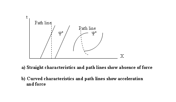
The relationship of the Lagrangian coordinate
system to the space-time coordinate system
is one of distortion; that is to say, it is a tensorial relationship.
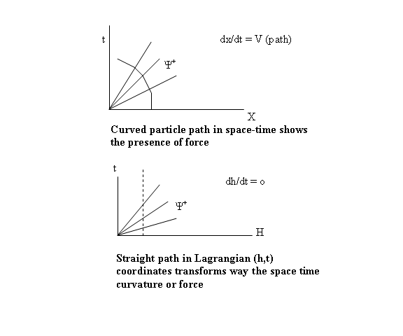
The transformation
h = x(h,t); h
= h)x,t)
(8)
between the two systems represents a distortion in the
relativistic, space-time, graphical representation. Here, dh = c dt = ds.
The analogous (tensorial) distortion of 4-space
(x,y,z,t) in general relativity – which is needed in order to obtain a
force-free representation- is valid, but ‘curved space-time’ is a graphical
concept only in compressibility terms, and has no physical foundation or
physical reality. The particle path curvature in 3-space is real; the absence
of curvature (force) in a Lagrangian system is a purely computational or
representational option, and its value is to be judged solely on its utility or
convenience, and not on any supposed insights it may offer into the nature of
physical reality.
The ‘force-free’ condition is
∫ds = ∫dh
= ∫c dt =0
(9)
In general relatatvity, ds , the geodesic arc element,
is
ds2
= ∑gijdxidxj
(10)
The fundamental equation of general relativity, needed
to gve force free motions, is therefore
δ∫
ds = 0
(11)
or, expressed as a tensor,
d2xμ/ds2 +
Г (dxμds)(dxν/ds) = 0
(12)
General relativity is a continuous field theory, and
as such, excludes discontinuities or singularities. Therefore, it appears to be fundamentally
incompatible with quantum physics, where we have shown shock discontinuities to
be the physical basis for the emergence of the particles of matter from
compressible energy flows (Sect. 3.9).
General relativity is compatible with the restricted
field of isentropic, classical mechanical motions, and of isentropic, optical
ray curvatures ( bending of light rays near gravitating masses).
Space-time coordinates arise from the introduction of
the relative velocity V in the compressible energy equation (1). So-called
space-time ‘warping’ is a coordinate effect, tat is to say it is a purely
graphical distortion in the depiction of an accelerated, compressible energy
flow.
General relativity is a valid computational means for
accelerated flows in a compressible field such as that of electromagnetic
radiation which has a finite signal speed.
But in the new quantum theory
of gravitation ( see Sect. 6.3), which is essentially beyond the space-time
‘event horizon’ of relativity, it would appear to be inapplicable.
6. GRAVITATION AND COSMOLOGY
6.0 Since the new theory has been successful in
reformulating quantum physics on a new basis and unifying it with relativity
theory, it is natural to apply it to gravitation. We shall now see that it offers a new quantum
theory of gravitation , and a new cosmology.
6.1 FORCE IN COMPRESSIBILITY TERMS
The basic compressibility force equation, expressed in
terms of wave and flow velocities is
F = dp/dt = mo/[1 – (V/co)2]1/2dV/dt
+ moV d[1 – (V/co)2]2/dt
= mo
(co/c) [a (1 + m2)]
(1)
where M = V/c is the Mach number of the flow, p is the
momentum, mo is the rest mass, a is the acceleration and c/co
is the Fitzgerald contraction factor ( Sect. 5.2.1).
If we set p = ε/c, we get
F = d(ε/c)/dt
F = 1/c dε/dt – (ε/c2) dc/dt
(1a)
6.1.1 ‘LONGITUDINAL MASS’
The long-standing puzzle of the so-called
‘longitudinal mass’ in relativity theory *Sect. 5.2.6), namely,
m = mo[1- (V/co)]1/2
(2)
no longer remains.
There is only one (relativistic) mass, which is
m = mo(c/co)
(3)
Instead of mass, it is now force which has a
compressibility correction term in the square of the Mach number M2,
and it can also be shown that it is this correction which introduces the 3/2
power factor in Eq.2 when the velocity and the acceleration are not co-linear.
6.1.2 FORCE IN PRESSURE GRADIENT TERMS
F = - 1/ρ dp/dx ( = 1/ρ Ñp, in general)
(4)
For n = 1 (k = 3):
Fp = 1/3 (c2/p) Ñp: p =
1/3 ρc2
For n = 2 (k = 2)´
Fp = 1/2 (c2/p) Ñp: p = 1/2 ρc2
6.1.3 WAVE SPEED,
C
c2 = k p/ρ = (n+2)/n p/ρ
(5a)
where 1/ρ = v = c2/kp, and so
c2 = co2 –V2/n
= k p/ρ
(5)
6.2 DERIVATION AND DIMENSIONS OF THE
GRAVITATIONAL CONSTANT G
From Sect. 3.5 and 3.6, where we introduced the
electromagnetic vibrational energy εh at a point in space (
i.r. for a particle), we saw that
Εh = cV = hν (6)
Now, for gravitational energy εg
attracting over the space intervening between masses, we can, by symmetry,
write
Εg = cV = Gk
(7)
where k = 1/λ is the wave number in tht space.
If cV is the same in both Eqs. (6) and (7), then
Εg/εh = cV/cV = 1 =
Gk/hν
(G/h) (k/ν) = 1
G/(h λν) = G/hc = 1
G/h = c (8)
Where G has the dimensions of energy times length.
This can be compared with Planck’s constant h ,which has dimensions of energy
times time.
On the above derivation, Planck’s constant has a
relationship to vibrational energy-density at a point in time via he frequency
ν ( h = cV/ν); whereas the gravitational constant G relates to an
energy-density at point in space between gravitating masses via the wave length
λ (G = cV/λ).
6.2.1 GRAVITATIONAL WAVE SPEED
If we now insert the numerical values for h and G in
(8), we get for the wave speed c
C = G/h = (6.67 x 10⁻¹¹)(6.63 x 10-34
= 1023 m/s)
(9)
This raises the question: Can such an enormous wave
speed be possible?
To answer, we plot the ordinary, compressible wave
speed’s energy (c2) from the
basic energy equation
c2 = co2 – V2/n
(5)
where we have the familiar energy ellipse in quantum
variables c and V, or the linear plot in energy variables c2 and V2:
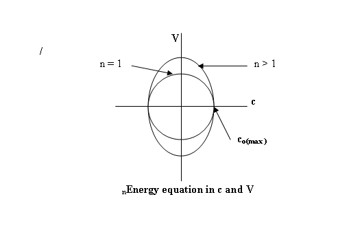
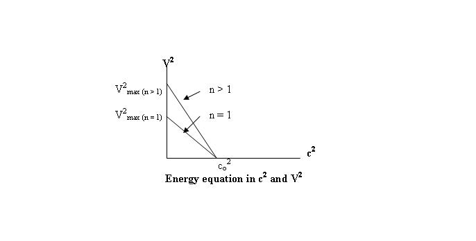
Here, co is 3 x 10¹⁰ m/s; the maximum
flow speed is Vmax = n1/2 co. But, if in the
energy equation (5), we now put n as being negative, then we have
c2 = co2 – V2/(-n)
= co2 + V2/(+n)
(10)
which plots as
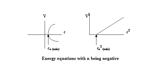
Here, with n being a negative quantity, co2
becomes a minimum wave speed ( = 3 x 10⁸ m/s, and there is no upper limit to either c or V.
The enormous wave speed ( c = 1023 m/s) indicated
in Eq. (9) is therefore compatible with an energy equation where n is a
negative quantity (Eq. (10). Furthermore, we see that , in variables c and V,
this plots as an hyperbola, instead of the usual energy ellipse.
Further support for the new wave speed will be found
in Sect. 6.8 in connection with the solution to the problem of the cosmological
constant.
Next, we seek a physical basis for this extraordinary
wave speed.
6.3 THE GRAVITATIONAL QUANTUM OR GRAVITINO
We have shown in Sect. 3.9 that ordinary matter is a condensed energy
form related to the entropy-associated variable n through the factor [n+1)]1/2,
where the number of degrees of freedom in the basic, steady-sate, energy
equation (5) is a positive integer: this energy equation is also elliptical in
the quantum state variables c and V.
However, in our new formulation of quantum mechanics
on the basis of compressible energy ( Sect. 3.6), we alsofound an ‘estra’
energyi term 2cV which afrises from either (a) the unsteady=stste energy
equation
c2 = co2
– V2/n – 2cV/n
which is also elliptical when rearranged to
c2 + V2/n + 2cV/n = co2 (elliptical)
or, (b) from squaring the quantum wave function to
obtain the energy
ψ2 = (c + iV)2 = c2
– V2/n + 2icV/n
ψ*2 = (c – iV/n)2 = (c2
+ V2/n) – 2icV/n
Now, if n is taken to be a negative ineger,then the
unsteady-state energy equation becomes
c2 +
V2/(-n) + 2cV/(-n) = co2
c2 – V2/n – 2cV/n = co2
(hyperbolic)
Since the cV ‘extra’ energy term can appear in either
an elliptical energy relationship or in the hyperbolic form, therefore, our
derivation of Eq. 3 ( and hence also Eq. 4) from the same cV term is
justified. Also, recalling that the cV
term generates all of the fundamental quantum relationships ( Sect. 3.60, it is
not unreasonable that it should also generate the gravitational constant G, as
we have suggested above – only now in a context of a hyperbolic energy equation
rather than the standard elliptical one.
As to a physical basis for this extraordinary
hyperbolic speed, we recall that the process of generation of the proton and
electron ( Sect. 3.12) also yields a stable, infinitely low-amplitude, pressure
balancing, rarefaction energy wave (R).

We propose that the rarefaction energy wave R must be
governed by the hyperbolic energy equation (1), and that this rarefied particle
is the gravitational quantum or gravitino, which we shall designate by νg. For its energy, we put
εg = G k = cV
(7)
(analogously to hν = vV)) but with c now given by
the hyperbolic energyi equation (10).
c2 = co2 - V2/(-n)
(10)
c2 =
co2 + V2/(+n)
This grounds the speed of the gravitino as being
either the wave speed c ( = 1023 m/s), or the flow speed V ( = 1023
m/s0. Such an enormous speed for the rarefaction energy form that we have here
called the gravitino νg. the carrier of the force of gravity,
would mean that gravitational influences in the universe are
quasi-instantaneous, since, at such a speed, the gravitational force would
cross the entire cosmos in a mater of minutes.
Newton’s hypothesis of instantaneous gravitational
interaction is thus supported by this conclusion. If this is so, then Galilean, and not
Lorentzian or relativistic relationships, would govern gravitational signals.
To conclude: the energy of a quantum wave function has
a 2cV term. In the case of ordinary elliptic energy, the emitted
electromagnetic radiation ( photon) is a compressed energy wave form; in the
case of hyperbolic energy, the 2cV term gives rise instead to a rarefied energy
emission, or rarefied particle, the quantum of gravity or gravitino νg.
Gravitational force thus arises from the tield of
rarefied energy gravitinos which are continuously generated and emitted by
elementary particles of matter ( Sect. 3.14) at a speed of 1023
m/s. The gravitational field now
consists of the massless gravitinos setting up a gravitational pressure
gradient which affects all elementary massive particles.
In effect, we have generated the gravitino by
quantizing the energy field cV/(-n) in a ‘space-like’ manner by inserting the
wave number or ‘inverse length’ in the formula Gk = cV; this arises from
symmetry considerations of the frequency or ‘time-like’m quantization of the
same field in the electromagnetic case by the Planck relationship for the
photon ε = hν = cV.
(Note that the speed of rarefied particles in general,
including neutrinos, need not be 1023 m/s, since from Eqn. (10), the
wave speed can vary from the minimum value of 3 x 10⁸ m/s on up to
infinity).ρ
6.4 THE FORCE OF GRAVITY IN COMPRESSIBILITY
TERMS
Newton’s graotational force equation
F = G m1m2/ r2
(11)
can be derived in terrms of compressible energy
parameters, namely the relative flow velocity V, and the pressure p, as
follows:
F = - 1/ρ dp/dx
(12)
=
(m) a = (m) dV/dt
= - 1/ρ
d(ρc2/k)/dx = - d(c2)/dx
provided that dρ/dx is small.
If c = U, the gravitational potential, then we have
Fg = -dU/dx = - - G(m1m2)/r2
= -1/ρ dp/dx
(13)
which in general gives
Fg = -1/ρ Ñp.
This gives the gravitational force in terms of the
pressure and density of a gravitino pressure field. Gravitational force,
therefore, appears to be analogous to a pressure gradient force.
In terms of the usual Newtonian equation of motion
for a gravitational field we have
Qr = (m) fr = Fμ
= V/cv (1/ρn) Ñp = V/c (1/ρn) Ñp = V/c (1/ρn) dp/dx
(14)
Here, V/v the Mach number of the energy flow, acts as
a force coupling constant; the
acceleration is denoted by fr, and Qr and Fμ
are forces.
6.5 EXCLUSIVELY ATTRACTIVE NATURE OF GRAVITY
In the above force equation (12), the negative sign
may be interpreted as a unidirectional force, that is a force of attraction.
Furthermore, on a physical basis, so long as the wave
acceleration (dc/dt) inside the gravitating mass particle is positive, the
entry of a rarefaction gravitino into the particle must decrease the energy
density. From the wave speed equation
c2 = k p/ρ
(5)
we see that such an energy density decrease must cause
an increase in the wave speed c: from Newton’s thir Law there will then beset
up an equal and opposite force towards the source of the absorbed gravitino,
that is to say, there will be a force of attraction.
6.6 A NEW FORCE LAW
In compressibility terms, we have
Fr = - dU/ds = -ÑU = - 1/(nρ) V/c Ñp
Ñ2U = Ñ× [1/(nρ) V/c Ñp ] = -4πG (m)
(Poisson equation)
Ñ2U =
0 (Laplace equation)
In relativistic terms, for a continuous, perfect
fluid, we have
Tμν….,ν + ρoFμ
= 0
Ρo is an invariant proper density, and
Fμ a world force vector.
The field equations of general relativity
Gλσ = -8πρλσ
could also be employed , if desired, (but see Sect.
6.12 regarding the ‘dark matter’ of the cosmos).
6.7 EQUIVALENCE OF GRAVITATIONAL AND INERTIAL
MASS: MACH’S PRINCIPLE
In the new theory, the equivalence principle becomes one
of force equivalence, rather than the equivalence of gravitational and inertial
mass as before. All force becomes
gravitational in the sense that all force arises from acceleration with respect
to the same background gravitino pressure field.
Because of the enormous gravitino speed ( c = 3 x 10²³
m/s), the local energy density is always in balance with, and can be related
to, the total mass of the universe.
Mach’s Principle is clearly complied with, although now on a new, and
physical basis.
We can see this more clearliy from the energy equation
c2 = co2 – V2/n
(5)
For constant energy (c2), the term V2/n
must also be constant. If V changes (
i.e. if there is acceleration) then energy must be supplied to or released from
the system. Thus necessary input or
export of energy is the source of inertia in the new theory, and the rate of
this energy lflow is the measure of force.
Mass is governed by – indeed, is generated by- the
factor [n+1]1/2 (Sect. 3.9), and so, for gravitational mass to
differ from the inertial mass, n would have to change. Therefore, for a particle of mass m, with n
being constant, we have
minertial = mgravitational
The force causing the curvature of the water surface
in Newton’s celebrated rotating water bucket experiment , thus arises from the
energy flow or acceleration with respect to the universal background gravitino
field; the latter now replaces Berkeley’s ‘fixed stars’ as a background reference;
this also essentially agrees with Mach’s Principle, but now, for the first
time, on a physical basis.
Note that, since V in the energy equation is purely
relative, the new theory is fully relativistic.
The theory, however, becomes quasi-Galilean for the case of gravitational radiation. Here, the relativistic corrections are now
negligible because of the enormous gravitino speed which gives
quasi-instantaneous signals cross the entire cosmos.
6.8 THE PROBLEM OF THE COSMOLOGICAL CONSANT
The cosmological constant Λ is given by Λ = (8π G ρv(/co2), where
ρv is the vacuum energy density.
Friedmann’s calculations in general relativity theory
led to the conclusion that Λ = 0. Quantum
field theory concludes that the vacuum energy density must, however, be between
1029 and 1046 J/m3. But astronomical observations agree with the
Friedmann conclusion that Λ must be zero.
The conflict between quantum physics and astronomical observations lies
in the enormous difference-ratio of 1046. This conflict is now resolvable in the new
theory through the new and enormous gravitino wave speed of 1023
m/s, since
Ε = co2 – [1023]2
= 1046 J/kg
That is to say, the estimates of the vacuum energy
density arising from standard quantum theory are in fact correct, but the
energy is not our ordinary, measurable, elliptic energy. Instead, it is a
rarefied or hyperbolic condensation of energy, and this is ordinarily undetected
in our condensed-energy material world.
The conflict in the estimates of the value of the cosmological constant
is thus resolved by the new theory – the value of Λ is zero.
6.9 THE FLATNESS PROBLEM: Ω EQUALS UNITY
In the expanding universe (Big Bang model), the ratio
of the initial gravitational energy to the initial kinetic energy of expansion, denoted by
Ω, determine whether the universe is open ( Ω < 1), closed (
Ω > 1) or ‘flat’ (Ω = 1).
In general relativity , these three criteria correspond to whether
space-time is hyperbolic, elliptical, or Euclidean (flat). In Sect. 6.2 we have put
(radiated kinetic energy) εh = hν = cV
(6)
(gravitational energy) εg = Gk = cV (7)
Both cV energies are generated in the same physical
process, namely, the interaction of two quantum wave functions,
characteristics, or enrays (Sects. 6.3;
4.1.1; 3.13). There is no
theoretical reason why this same equality of kinetic and gravitational energies
in Eqs. (6) and (7) should not also apply at the Initial Event of creation, and
so the new theory states that the value of Ω is always unity. The universe is therefore ‘flat’ or
Euclidean.
6.10 ACTION-AT-A-DISTANCE: THE ASPECT et al.
EXPERIMENTS
The quantum wave function’s extra-energy term (2cV)
which is involved with the fast moving gravitino, is generated and emitted in
the same process which is also the source of the emission of the electromagnetic
quantum or photon. The former, of
course, must then contain the same phase and momentum information as the
latter, that is, the gravitino emitted at 1023 m/s contains the same
quantum information as the photon emitted at 3 x 10⁸ m/s.
The experiments of Aspect et al. confirming the
universal and instantaneous spread of wave function information are now
explainable by the 2cV phase, momentum and polarization information carried by
the gravitino at quasi-instantaneous speed to the detecting apparatus, well
ahead of the same information carried by the slow-moving photon.
6.11 THE HIDDEN MASS,OR ‘DARK MATTER’ OF THE
UNIVERSE: A NEW SOLUTION
Currently, the observed astronomical motions of certain
structures of the universe, such as galaxies and clusters, can be explained by
Newton’ laws of motion only with the assumption that there is present in and
around the structures additional ‘hidden’ , unobservable, or ‘ dark matter’
amounting to from 90% to as much as 99% of the total mass of the universe; the optically and electromagnetically
observed mass, therefore, constitutes only from 10% to as little as 1% of the
total mass required to explain the motions.
The existence and nature of this dark matter is a central problem of
cosmology today.
Now in the new theory, we have assigned the force of
gravity to a pressure field of massless, gravitinos, which are continuously
emitted during the unceasing formation and reformation of the quantum wave interaction
which generates the elementary particles of mater and stablizes their existence
(Sect. 3.14).
Because the rarefied gravitino has such an enormous
speed, it easily escapes the shock wave which encases and stabilizes all
elementary particles, and it then speeds out across the universe. Since this gravitino does not itself emit
gravitinos, it cannot be the source of the hidden mass, and so we must look
further.
6.11.1 THE EQUATION OF STATE HAS TWO FORMS
The equation of state for compressible energy has not
just one, but two possible forms:
A) pv = RT (isothermal); kpv = RT ( adiabatic)
(15)
p2/a2 –v2/b2
= const. (hyperbolic)
B) p2/a2 + v2/b2
= const. (elliptical)
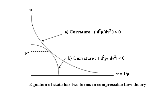
In World A: (d2p/dv2)s
> 0. Compression waves (condensed
energy waves) steepen with time to form compression shocks, and these in turn
form th elementary particles of matter.
Rarefaction waves, on the other hand, die out, and only infinitely low-amplitude
rarefaction waves, such as the gravitino νg can exist (Sect.
2.11).
In World B: (d2p/dv2)s
< 0). Rarefaction waves ( rarefied energy waves) steepen to form rarefaction
shocks. Compression shocks would die out, and only infinitely low-amplitude
compression waves would exist.
In all known material, compressible fluids only
compression waves can exist, and n, the number of degrees of freedom parameter,
is positive. Rarefaction states in a
World B would, therefore, necessarily have n negative.
6.11.2 RAREFIED OR CELESTON MATTER
Rarefaction shocks in World B would form rarefied,
elementary particles ( which we shall
designate celestons).
These are the counterparts to the baryons, mesons and
leptons of out World A of condensed energy forms . ( The electron-neutrino
νe, muon-neutrino νμ and tau-neutrino
ντ may possibly be already known examples of World B
particles).
We now propose a transformation from World A matter to
World B matter. This transformation A→
B takes place at a critical pressure p* ( see Figure page xx). Because of an entropy relationship
ΔSA = Δn/(+n); and
ΔSB = Δn/(-n)
The transformation A → B, once begun, would be
irreversible.
At an Initial or Creation Event ( e.g. a Big Bang) in
a compressible expanding universe we would have p >>>p*, and so only
condensed elementary particles of World A matter could emerge.
World B (rarefied or celeston matter) could only form
when the critical pressure p* was reached.
This point, however, might be reached locally (for example, in the centre of a vortex where the pressure
is lower) before the expansion of the universe had reduced the overall cosmic
pressure to the critical value p*.
The Initial Event would usher in a Unitary World A of
condensed matter only ( p > p*) . Our present era (p ≥ p* ) is that of
a Binary Universe ( A + B) where both compressed and rarefied energy forms
of matter can exist.
A final cosmic state ( p < p*), which will begin
when the overall cosmic pressure falls to the critical value, will again usher
in a Unitary universe, but this time it will consist of World B, rarefied, or
celeston matter only.
The gravitino νg would be the simplest
possible rarefaction wave form, or celeston. How the graviton relates to the electron-neutrino,
or to the muon-neutrino is a matter for study by quantum specialists, as is
also the further theoretical investigation of the various possible other types of celeston
particles which might be generated by a rarefaction shock process using
negative values for the entropy parameter n.
The scientific grounding of such a theory would necessarily rest on
astronomical data ( See Sects. 6.11.4 and 6.11.5).
6.11.3 LOCAL PRESSURE LOWERING IN VORTICES
The pressure is given by
p = po - ò (ρw2/r)
dr, or
p = po
- ρò (w2/r) dr
The core pressure
pc is given by
pc= po – (ρw2)/8π2r2
The compressible vortex ratios are:
Vmax / r* = c*/rmin =
[(k-1)/(k+1)]1/2 = [ 1/(n+1)]1/2
r/r* = 1/(V/c*)
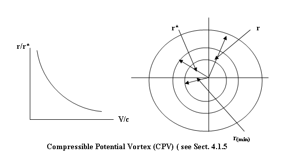
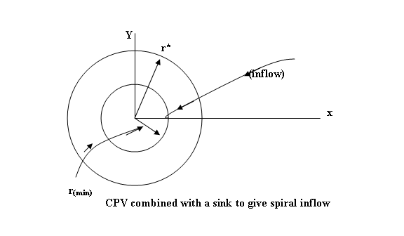
The transformation of ordinary matter via the process
A → B at r*. produces the necessary sink for continuous spiral inflow,
because the matter flowing in to the vortex core is transformed from ordinary
World a matter to the celeston or rarefied matte of World B.
(The ‘event horizon’ of general relativity’s black
hole theory might correspond roughly to our
rmin.).
6.11.4 QUASARS IN EARLY COSMIC TIMES (P >>
P*)
Local pressure lowering in vortices in the early
universe would not permit the pressure to drop sufficiently for p to reach
p*. In this case, with no A → B
effect, the sink causing the pressure lowering would have to be due to some
process such as divergent flow.
Inflowing A-matter would be subjected to very large
dynamic and thermodynamic effects near the quasar’s critical radius r*, and
would therefore radiate strongly, but the A-matter would not transform to the
B-state. Thus, quasars could form in the
primitive universe, as is observed.
6.11.5 SPIRAL AND ELLIPTICAL GALALXIES (PLOC
< P*)
With an overall pressure lowering due to cosmic expansion,
at some later time in cosmic history the pressure in the core of a vortex would
drop to the critical pressure p*, and the transformation to B=matter could then
take place locally.
In such cases, the
central core would become a (transformation) sink. Quasars, having no such sink, could not
persist; instead, spiral and elliptical galaxies with central sinks would
emerge as the dominant cosmological structures.
Transformations of A-matter ( condensed, ordinary
matter to World B matter ( rarefied, celeston matter) then would take place in
the galactic cores. The ‘dark matter’
produced in the vortex core then would expand and spread throughout the galaxy
producing a ‘halo’ of ‘dark matter’ as is observed. The universe is then in a binary state ( A +
B).
The model can readily be extended to include the
observed distinction between active and normal spirals.
6.12 EXPERIMENTAL TEST OF THE PROPOSED A →
B TRANSFORMATION: QUASARS VS. GALAXIES
In the new theory, the change from quasar abundance in
the early universe to their replacement
by spiral and elliptical galaxies reflects and marks the critical pressure p*
which controls the A → B transformation process just described.
Quasars, having no B or ‘dark matter’ should then have
their experimentally observed motions explainable by Newton’s laws of motion
using only their optically or electromagnetically observable mass; this
prediction should, in principle, be open to experimental testing.
The energy change ΔE in the transformation A →
B is given from the energy equations
ΔE = cB2 – cA2
= V2[ 1/nA – 1/nB]
Since nA is positive and nB is
negative, energy must be evolved in the A → B transformations.
It might, therefore, be possible to calculate the
energy evolved in galactic transformations of he type A → B from the
above equation, that is to calculate the energy released the process of
production of the proposed celeston matter from our ordinary condensed World A
matter in the vortex core of a galaxy.
Thus might be another experimental test of the A→ B
transformation.
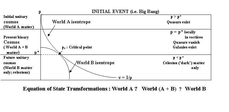
SELECTED
BIBLIOGRAPHY
COMPRESSIBLE FLOW
Shapiro, A.H., The
Dynamics and Thermodynamics of Compressible Fluid Flow.2 vols., J
John Wiley & Sons, New York, 1953.
Courant, R., and Friedrichs, K.O., Supersonic Flow and Shock Waves.
Interscience, New York, 1948.
Lamb, Horace, Hydrodynamics.8th
ed., Cambridge University Press, 1932.
Morse, P.M., Vibration
and Sound. McGraw-Hill, New York, 1948.
Tietjens, O.G/, Fundamentals
of Hydro- and Aeromechanics, (based on the lectures of L.Prandtl). McGraw Hill, 1969. Deve reprint, New York,
1957.
Rayleigh, J.W.S., The
Theory of Sound. 2 vols. 1886. Dever reprint, New York 1945.
QUANTUM PHYSICS
Ziman, J.M., Elements
of Advanced Quantum Theory. Cambridge University Press, 1969.
Sudbery, A., Quantum
Mechanics and the Particle of Nature. Cambridge Universityi Press, 1986.
Van der Waerden, B.L., (ed.), Sources of Quantum Mechanics. Dovefr, New York,1949.
Heisenberg, W., The
Physical Principles of the Quantum
Theory. 1939. Dever reprint, New York, 1949.
Penrose, R. and Rindler, W., Spinors and Space-time. Vol .1, Two-spinor Calculus and Relativistic fields. Cambridge University Press, 1984.
Planck, Max, Theory
of Heat Radiation, 2nd ed. 1913.
Dover reprint, New York, 1959.
RELATIVITY
Bergman, P.C., Introduction
to the Theory of Relativity, Dover reprint, New York, 1976.
Pauli, W., Theory
of Relativity (1921), Dover reprint,
New York, 1981.
Einstein,A., Lorentz, H.A.,Weyl, H, and Minkowski,
H.J., The Principle of Relativity ( (Collection of original
memoirs on the Special and General Theory of Relativity with Notes by A.
Sommerfeld). Dover reprint, New
York.1952.
Morse, P.M., and Feshbach, H., Methods
of Theoretical Physics.2 vols. McGraw Hill, New York, 1953.
MECHANICS, GRAVITATION AND COSMOLOGY
Lindsay, R.B., and Margenau, H., Fundamentals of Physics. Dover reprint, New York, 1957.
Menzel, D.H., Mathematical
Physics, Dover reprint, New York, 1961.
Power, B.A., Shock
Waves in a Photon Gas, Contributed Paper No.203, American Association for
the Advancement of Science, Annual Meeting, Toronto, Jan.1981.
___________, Unification
of Forces C. and Particle Production at an Oblique Radiation Shock, Contr. Paper No. 462, American
Association for the Advancement of Science, Annual Meeting, Washington, D.C.,
Jan. 1982.
__________, Baryon Mass-ratios and Degrees of Freedom in
a Compressible Radiation Flow. Contr.
Paper No. 505, American Association for the Advancement of Science, Annual
Meeting, Detroit, May 1963.
___________, Gravitation: An Energy Compressibility Effect.
Monograph, July 1983.
____________, Prediction
of Elementary Particle Mass-ratios from Compressible FlowTheory. Monograph,
May 1985.
Menzel, D.H., (ed) Fundamental
Formulas of Physics. 2 vols.,
Dover, New York, 1960.
![]()
Copyright, Bernard A.
Power, September 1992